Tutorial on use of intraclass correlation coefficients for assessing intertest reliability and its application in functional near-infrared spectroscopy–based brain imaging

Lin Li; Li Zeng; Zi-Jing Lin; Mary Cazzell; Hanli Liu

doi:10.1117/1.JBO.20.5.050801

20 May 2015 Tutorial on use of intraclass correlation coefficients for assessing intertest reliability and its application in functional near-infrared spectroscopy–based brain imaging

Lin Li, Li Zeng, Zi-Jing Lin, Mary Cazzell, Hanli Liu

Author Affiliations +

Journal of Biomedical Optics, Vol. 20, Issue 5, 050801 (May 2015). https://doi.org/10.1117/1.JBO.20.5.050801

Abstract

Test-retest reliability of neuroimaging measurements is an important concern in the investigation of cognitive functions in the human brain. To date, intraclass correlation coefficients (ICCs), originally used in inter-rater reliability studies in behavioral sciences, have become commonly used metrics in reliability studies on neuroimaging and functional near-infrared spectroscopy (fNIRS). However, as there are six popular forms of ICC, the adequateness of the comprehensive understanding of ICCs will affect how one may appropriately select, use, and interpret ICCs toward a reliability study. We first offer a brief review and tutorial on the statistical rationale of ICCs, including their underlying analysis of variance models and technical definitions, in the context of assessment on intertest reliability. Second, we provide general guidelines on the selection and interpretation of ICCs. Third, we illustrate the proposed approach by using an actual research study to assess intertest reliability of fNIRS-based, volumetric diffuse optical tomography of brain activities stimulated by a risk decision-making protocol. Last, special issues that may arise in reliability assessment using ICCs are discussed and solutions are suggested.

1. Introduction

Test-retest reliability is one of the basic aspects in the examination of scientific measurements and physiological or psychological quantifications. In the field of behavioral sciences, the intraclass correlation coefficient (ICC) has been a common parameter or index used to estimate measurement reliabilities induced by human errors and variations among judges or raters. Shrout and Fleiss reviewed a class of ICCs and provided guidelines for use in inter-rater reliability in behavioral sciences research.¹ McGraw and Wong gave a more complete review of various forms of ICC and inference procedures in the same context for behavioral sciences research.² Weir discussed issues in the use of ICCs for quantifying reliability in movement sciences.³ These studies provided a statistical foundation for reliability assessment and emphasized that there are different forms of ICC, which may lead to different results when being applied to the same data. Therefore, it is important to choose an appropriate form of ICC which matches with the experimental design and concerns in a specific study.

In the neuroimaging field, numerous groups have adapted different forms of ICC for assessing test-retest reliability in different applications of functional brain imaging. For example, Plichta et al. and Bhambhani et al. applied ICC(1,1) and ICC(1,2) in quantification of test-retest reliability in functional near-infrared spectroscopy (fNIRS) studies.⁴^,⁵ Braun et al. used ICC(3,1) and ICC(2,1) to study the reliability of a functional magnetic resonance imaging (fMRI)-based graph theoretical approach.⁶ Table 1 lists a few examples of recently published papers on fMRI and fNIRS studies, where ICCs were used to measure test-retest reliability.

Table 1

Examples of functional near-infrared spectroscopy (fNIRS)/functional magnetic resonance imaging (fMRI) reliability studies using intraclass correlation coefficients (ICCs).

References	Modality	ICC type	Topic of measurement
4	fNIRS	Not provided	Handgrip exercise in healthy and traumatic brain-injured subjects
5	fNIRS	ICC(1,1), ICC(1, $k$ )	Visual stimulation by a period of checkerboard
7	fNIRS	ICC(1,1), ICC(1, $k$ )	Motor cortex stimulation by finger tapping
8	fNIRS	ICC(1,1), ICC(1, $k$ )	aResting-state functional connectivity
9	fMRI	ICC(1,1), ICC(1, $k$ )	bResting-state brain networks
10	fMRI	ICC(3,1)	Combination of an emotional, a motivational, and a cognitive task
6	fMRI	ICC(2,1), ICC(3,1)	bResting-state brain networks
11	fNIRS	ICC(1,1), ICC(1, $k$ )	Repetitive transcranial magnetic stimulation
12	fMRI	ICC(2,1)	bResting-state brain networks
13	fNIRS	ICC(1, $k$ )	bResting-state brain networks
14	fMRI	ICC(2,1)	aResting-state functional connectivity
15	fMRI	ICC(2,1)	bBrain networks in working memory, emotion processing, and resting state

^aSeed-based analysis.

^bGraph-theory-based analysis.

There are two limitations for the listed studies. First, different forms of ICCs are used in these studies without reasoning the choice of selected ICC forms. As a result, it is not clear whether the chosen ICC metrics appropriately fit the study, and it will also be difficult to compare results among different studies. Second, most literature on ICCs is in the context of inter-rater reliability studies in which a set of targets are rated by several judges, while neuroimaging researchers are concerned about the intertest reliability of a certain image modality in repeated tests. No explanation on this essential difference is given in the literature.

Since the ICCs are derived under different assumptions, their values would be meaningful only if those assumptions are met. In addition, it is important and critical to correctly interpret results and draw inference when different forms of ICC are used to assess instrument-based intertest reliability. To our best knowledge, no work in the fNIRS field has been done to address those issues. In this paper, we wish to achieve three objectives: the first is to give a brief review and tutorial on the statistical rationale of ICCs and their application for assessment of intertest reliability; the second objective is to provide general guidelines on how to select, use, and interpret ICCs for assessing intertest reliability in neuroimaging research; the last objective is to assess intertest reliability of multichannel fNIRS under a risk decision-making protocol, as an example, to demonstrate the appropriate ICC-based reliability analysis.

The remainder of the paper is organized as follows. In Sec. 2, we first present the statistical rationale of ICCs, followed by guidelines in Sec. 3 on the selection of ICCs in test-retest reliability assessment. In Sec. 4, as a demonstrative and explicit example, we briefly introduce the methodology used and show hemodynamic images measured twice by multichannel fNIRS in response to a risk decision-making protocol using the Balloon Analog Risk Task (BART), followed by comprehensive ICC analysis and result interpretation. Finally, we will discuss several issues possibly encountered in ICC-based reliability assessment in Sec. 5, followed by conclusion in Sec. 6. While this study focuses on fNIRS-based functional brain imaging, it represents a common subject on test-retest reliability of neuroimaging measurements and, thus, has broad applicability to various neuroimaging modalities.

2. Intraclass Correlation Coefficient

Before utilizing ICCs for assessing test-retest reliability of fNIRS-derived brain images of oxygenated hemoglobin changes ( $Δ HbO$ ) and deoxygenated hemoglobin ( $Δ HbR$ ) recorded during a risk-decision task, in this section, we first introduce a unified analysis of variance (ANOVA) model as the statistical foundation of the ICCs (Sec. 2.1), then review the six forms of ICC that are commonly used in reliability assessment (Sec. 2.2), followed by clear descriptions of ICC criteria used to assess reliability of measurements (Sec. 2.3).

2.1.

Unified ANOVA Model

In order to assess test-retest reliability, data as shown in Table 2 are usually collected. Assume that $n$ subjects ( $j = 1, \dots, n$ ) are used in this study, and $k$ repeated tests ( $i = 1, \dots, k$ ; $k = 2$ for a test-retest case) are conducted on each subject. Let $y_{i j}$ be the recorded quantity of the $j$ ’th subject in the $i$ ’th test/measurement. Note that in the context of inter-rater reliability assessment, as considered in most ICC literature, a set of targets is rated by several judges; the reliability of the raters is determined. In contrast, in the context of test-retest reliability assessment, a set of subjects is measured in two or more repeated tests or measures; the intertest reliability of the tests is the characteristic the researcher will quantify. Thus, “subjects” and “tests or measures” in our study correspond to “targets” and “judges,” respectively, in the inter-rater reliability study.

Table 2

Dataa used in test-retest reliability assessment.

Test (i=1,…,k)	Subject (j=1,…,n)
Test (i=1,…,k)	j=1	j=2	…	j=n
1	$y_{11}$	$y_{12}$	…	$y_{1 n}$
2	$y_{21}$	$y_{22}$	…	$y_{2 n}$
…	…	…	…	…
$k$	$y_{k 1}$	$y_{k 2}$	…	$y_{k n}$

^aIn our study, yij represents fNIRS readings from the j’th subject in the i’th measurement.

Appropriate ANOVA models are the basis of ICCs. Equation (1) below expresses the unified ANOVA model for the data in Table 2:

Eq. (1)

y_{i j} = μ + S_{j} + T_{i} + e_{i j},

where

μ

is the overall population mean,

S_{j}

is the deviation from the population mean of the

j

’th subject,

T_{i}

is the systematic error in the

i

’th test, and

e_{i j}

is the random error in the measurement of the

j

’th subject in the

i

’th test. This model rests on the idea that the measurement is a combination of the true status of the subject (i.e.,

μ + S_{j}

) and measurement errors (i.e.,

T_{i} + e_{i j}

).³ Different systematic errors in the tests (i.e.,

T_{1}, T_{2}, \dots, T_{k}

) may be caused by different measurement conditions in the tests (e.g., different devices are used in the tests, or the tests are conducted at different locations or time slots) or the learning effects in repeated testing (e.g., subjects tend to become more and more skilled in later tests). The random error is the error due to uncontrollable random factors, such as patient factors, environmental factors, and operator errors.

Assumptions on each term in the model are as follows:

A1: Subject is a random factor and $S_{j}$ represents the random effect of this factor, which is assumed to follow a normal distribution with mean 0 and variance $σ_{S}^{2}$ :

Eq. (2)

S_{j} \sim N (0, σ_{S}^{2}) .

Here, the term random factor means that subjects involved in this study are viewed as randomly selected from a larger population of possible subjects. Accordingly, the variance $σ_{S}^{2}$ represents the heterogeneity among this population.

A2: Test can be treated as a random factor or a fixed factor, and $T_{i}$ is the systematic error in the $i$ ’th test. When it is treated as a random factor, $T_{i}$ represents the random effect of this factor, which is assumed to follow a normal distribution with mean 0 and variance $σ_{T}^{2}$ . When it is treated as a fixed factor, $T_{i}$ represents the fixed effect of this factor, and it is assumed that the sum of the effects is 0. Equations (3) and (4) explain these two effects in mathematical expressions:

Eq. (3)

Random effect : T_{i} \sim N (0, σ_{T}^{2}),

Eq. (4)

Fixed effect : \sum_{i = 1}^{k} T_{i} = 0 .

The difference between random factor and fixed factor is that in the former case, the repeated $k$ tests conducted in the study are viewed as random samples from a larger population of possible tests/measurements, and accordingly, the variance $σ_{T}^{2}$ represents the variability of this population. In the latter case, the repeated $k$ tests are not representative of possible tests; the concern is only the effect of these particular tests conducted in the study instead of a generalization to the underlying population of possible tests. Note that $T_{i}$ is a random variable in the case of random factor and a fixed, unknown quantity in the case of fixed factor.

A3: The random error is assumed to follow a normal distribution with mean 0 and variance $σ_{e}^{2}$ :

Eq. (5)

e_{i j} \sim N (0, σ_{e}^{2}) .

A4: The effect of interaction between the subject and test (i.e., $Subject \times Test$ ) is assumed to be insignificant and thus is ignored in Eq. (1). This means that the systematic error of each test is similar for all subjects, which is reasonable in most cases. In situations where this assumption is violated (i.e., the systematic error varies from subject to subject), this interaction effect is mingled with the random error and not identifiable using the data shown in Table 2 since there is no replicate under each combination of subject and test. In this case, the equations of ICCs are the same as in the case without the interaction effect.

Based on the unified ANOVA model, several special models can be obtained by adopting different assumptions regarding whether the effect of the test is significant and whether to treat the test as a random or fixed factor in A2 above. Different forms of ICC can be derived from those special models as shown in the following section.

2.2.

Six Forms of ICC

The ICCs reviewed by Shrout and Fleiss are based on three special models derived from the unified model: one-way random-effect model (model 1), two-way random-effect model (model 2), and two-way mixed-effect model (model 3).¹ These models are listed in Table 3. If we assume that the effect of test is not significant (i.e., systematic error is negligible or systematic errors in the repeated tests do not differ significantly), the term $T_{i}$ can be removed from the unified model, which leads to the one-way random-effect model. When the effect of the test cannot be ignored and the test is treated as a random factor given in A2 by Eq. (3), the unified model becomes a two-way random-effect model. If the test is treated as a fixed factor as given in A2 by Eq. (4), the unified model becomes a two-way mixed-effect model. The name ‘mixed effect’ comes from the fact that the model contains both random effect (i.e., $S_{j}$ ) and fixed effect (i.e., $T_{i}$ ).

Table 3

Analysis of variance (ANOVA) models as basis of ICCs.

Model	Form	Assumptions
One-way random-effect model	$y_{i j} = μ + S_{j} + e_{i j}$ $i = 1, \dots, k$ ; $j = 1, \dots, n$	$S_{j} \sim N (0, σ_{S}^{2})$ ; $e_{i j} \sim N (0, σ_{e}^{2})$ Systematic error of test is insignificant.
Two-way random-effect model	$y_{i j} = μ + S_{j} + T_{i} + e_{i j}$ $i = 1, \dots, k$ ; $j = 1, \dots, n$	$S_{j} \sim N (0, σ_{S}^{2})$ ; $T_{i} \sim N (0, σ_{T}^{2})$ ; $e_{i j} \sim N (0, σ_{e}^{2})$
Two-way mixed-effect model	$y_{i j} = μ + S_{j} + T_{i} + e_{i j}$ $i = 1, \dots, k$ ; $j = 1, \dots, n$	$S_{j} \sim N (0, σ_{S}^{2})$ ; $\sum_{i = 1}^{k} T_{i} = 0$ ; $e_{i j} \sim N (0, σ_{e}^{2})$

Table 4 shows the variance decomposition in each of the three models, including the degrees of freedom, mean squares (MS), and expected mean squares of each variance component. Specifically, in the one-way random-effect model, the total variance of measurements is decomposed into two components: between-subjects variance and within-subjects variance, which are estimated by the between-subjects mean squares ( ${MS}_{B}$ ) and within-subjects mean squares ( ${MS}_{W}$ ), respectively.

{MS}_{B} = \frac{k}{n - 1} \sum_{j = 1}^{n} {({\bar{y}}_{. j} - {\bar{y}}_{..})}^{2},

{MS}_{W} = \sum_{i = 1}^{k} \sum_{j = 1}^{n} {(y_{i j} - {\bar{y}}_{. j})}^{2},

where

{\bar{y}}_{. j}

is the mean of measurements on the

j

’th subject (i.e., data in the

j

’th column of Table 2), and

{\bar{y}}_{..}

is the mean of all the measurements across all the subjects in Table 2. In the two-way random-effect and mixed-effect models, the total variance is decomposed into three components: between-subjects variance, between-tests variance, and random error variance, which are estimated by the between-subjects mean squares (

{MS}_{B}

), between-tests mean squares (

{MS}_{T}

), and residual mean squares (

{MS}_{E}

).

{MS}_{B}

has the same equation as in the one-way random-effect model, and

{MS}_{T}

and

{MS}_{E}

are defined by

{MS}_{T} = \frac{n}{k - 1} \sum_{i = 1}^{k} {({\bar{y}}_{i .} - {\bar{y}}_{..})}^{2},

{MS}_{E} = \frac{1}{(n - 1) (k - 1)} \sum_{i = 1}^{k} \sum_{j = 1}^{n} {(y_{i j} - {\bar{y}}_{i .} - {\bar{y}}_{. j} + {\bar{y}}_{..})}^{2},

where

{\bar{y}}_{i .}

is the mean of measurements in the

i

’th test (i.e., data in the

i

’th row of Table 2). It is worth mentioning that the mean squares can be obtained automatically from the software output in ANOVA analysis.

Table 4

Variance decomposition in the ANOVA models.

	df	MS	EMS
One-way random-effect model
Between-subjects	$n - 1$	${MS}_{B}$	$k σ_{S}^{2} + σ_{e}^{2}$
Within subjects (error)	$n (k - 1)$	${MS}_{W}$	$σ_{e}^{2}$
Two-way random-effect model
Between subjects	$n - 1$	${MS}_{B}$	$k σ_{S}^{2} + σ_{e}^{2}$
Within subjects
Between tests	$k - 1$	${MS}_{T}$	$n σ_{T}^{2} + σ_{e}^{2}$
Error	$(n - 1) (k - 1)$	${MS}_{E}$	$σ_{e}^{2}$
Two-way mixed-effect model
Between subjects	$n - 1$	${MS}_{B}$	$k σ_{S}^{2} + σ_{e}^{2}$
Within subjects
Between tests	$k - 1$	${MS}_{T}$	$(n / k - 1) \sum_{i = 1}^{k} T_{i}^{2} + σ_{e}^{2}$
Error	$(n - 1) (k - 1)$	${MS}_{E}$	$σ_{e}^{2}$

Note: df, degree of freedom; MS, mean squares; EMS, expected mean squares.

The ICC is rigorously defined as the correlation between the measurements on a subject in the repeated tests.¹ Intuitively, if this correlation is high, that means the neuroimaging modality yields very similar measurements in the tests (or test and retest when $k = 2$ ), an indicator of high reliability. A more technical interpretation of ICC is that it is a measure of the proportion of variance due to subjects² among the total variance. Following this interpretation, ICC can be further defined into two categories: as measure of test (absolute) agreement and as measure of test consistency.² Equations (6) and (7) are the expressions of the two definitions:

Eq. (6)

Reliability (Agreement) = \frac{Between- subjects variance}{Between-subjects variance + Between -tests variance + Random error variance},

Eq. (7)

Reliability (Consistency) = \frac{Between -subjects variance}{Between - subjects variance + Random error variance} .

For each of the three models, the reliability of a single measurement and reliability of the average of the $k$ measurements (called the reliability of the average measurement for simplicity hereafter) will be considered. This gives a total of $3 \times 2 = 6$ possible forms of ICC. The six forms of ICC developed by Shrout and Fleiss, which have been widely used in the literature, are summarized in Table 5.¹ Following the notations in the primary reference,¹ these ICCs are designated as ICC(1,1), ICC(1, $k$ ), ICC(2,1), ICC(2, $k$ ), ICC(3,1), and ICC (3, $k$ ), where the first index indicates one of the three underlying ANOVA models (see Table 3), and the second index indicates whether the reliability of a single measurement ( $= 1$ ) or that of the average measurement (over $k$ repeated tests) is considered.

Table 5

Definition of ICCs and computation equations.

Designation	Model	Definition	Computation formula
ICC(1,1)	One-way random-effect model	$σ_{S}^{2} / σ_{S}^{2} + σ_{e}^{2}$	${MS}_{B} - {MS}_{W} / {MS}_{B} + (k - 1) {MS}_{W}$
ICC(1, $k$ )	One-way random-effect model	$σ_{S}^{2} / σ_{S}^{2} + σ_{e}^{2} / k$	${MS}_{B} - {MS}_{W} / {MS}_{B}$
ICC(2,1)	Two-way random-effect model	$σ_{S}^{2} / σ_{S}^{2} + σ_{T}^{2} + σ_{e}^{2}$	${MS}_{B} - {MS}_{E} / {MS}_{B} + (k - 1) {MS}_{E} + k {(MS}_{T} - {MS}_{E}) / n$
ICC(2, $k$ )	Two-way random-effect model	$σ_{S}^{2} / σ_{S}^{2} + (σ_{T}^{2} + σ_{e}^{2}) / k$	${MS}_{B} - {MS}_{E} / {MS}_{B} + {(MS}_{T} - {MS}_{E}) / n$
ICC(3,1)	Two-way mixed-effect model	$σ_{S}^{2} / σ_{S}^{2} + σ_{e}^{2}$	${MS}_{B} - {MS}_{E} / {MS}_{B} + (k - 1) {MS}_{E}$
ICC(3, $k$ )	Two-way mixed-effect model	$σ_{S}^{2} / σ_{S}^{2} + σ_{e}^{2} / k$	${MS}_{B} - {MS}_{E} / {MS}_{B}$

Note: σe2=MSE, σS2=MSB−MSE/k, and σT2=MST−MSE/n.

2.3.

ICC Criteria to Assess Reliability of Measurements

Since ICCs measure a correlating relationship with a value between 0 and 1, it is practically important to have standard criteria used to assess the reliability of measurements. According to published literature,¹⁶^,¹⁷ criteria of ICC values for medical or clinical applications are grouped into four categories, listed as follows. The level of clinical significance is considered poor, fair, good, and excellent when $ICC < 0.40$ , $0.40 < ICC < 0.59$ , $0.60 < ICC < 0.74$ , and $0.75 < ICC < 1.00$ , respectively. In the present study, we follow the same criteria since most of the previous publications in the neuroscience field have utilized the same or very similar criteria.⁶^,⁸^–¹⁰^,¹⁵^,¹⁸^,¹⁹ Note that different applications may vary the ICC range to a large extent based on specific needs and definitions given by individual clinical applications.²⁰^,²¹ In general, using $ICC = 0.40$ as the floor of an acceptable range for the reliability of measurements is still reasonable as most fMRI results have ICC values of 0.33 to 0.66,²² which are commonly considered reliable.

3. Selection of ICCs

One critical issue or puzzle in applying ICCs to assess the reliability of neuroimaging measurements is how to select appropriate ICCs from the six forms given in Table 5 for a specific study. How to make an appropriate selection is the topic of this section. We will first present several properties on the interpretations and magnitudes of the ICCs and then provide detailed guidelines on ICC selection.

3.1.

Properties of ICCs

The six forms of ICC given in Table 5 have the following properties:

Property 1: ICC(1,1)/ICC(1, $k$ ) and ICC(2,1)/ICC(2, $k$ ) are measures of test agreement [i.e., as defined by Eq. (6)] as the between-tests variance is included in their denominators; ICC(3,1)/ICC(3, $k$ ) are measures of test consistency [i.e., as defined by Eq. (7)] as the between-tests variance is not included in their denominators.

Property 2: Among the three ICCs for a single measurement, the relationship of ICC(1,1) $\leq ICC (2,1)$ $\leq ICC (3,1)$ exists in most cases. Specifically, when the effect of test is not significant, namely, $σ_{T}^{2}$ is small, these three ICCs have similar values as their denominators are close to each other [see Eqs. (6) and (7)]. When the effect of test is significant, the correlation between measurements will be underestimated in the one-way random-effect model,¹ that is, ICC(1,1) $< ICC (2,1)$ . In this case, we expect that ICC(2,1) $< ICC (3,1)$ because the denominator of ICC(3,1) does not include the between-tests variance and, thus, is smaller than that of ICC(2,1).

Property 3: ICCs of the average measurement are larger than their counterparts of a single measurement. The reason is that averaging over repeated measurements reduces the variance of measurement/test errors, leading to a decrease in between-tests variance and an increase in overall ICCs, as interpreted by Eq. (6).

3.2.

Guidelines on ICC Selection

To appropriately assess reliability of neuroimaging measurements, appropriate ICCs need to be chosen based on the specific study. Usually both the ICC of a single measurement and that of the average measurement will be used, so the primary issue here is how to choose the most appropriate ANOVA model among the three alternatives: model 1 (one-way random-effect model), model 2 (two-way random-effect model), and model 3 (two-way mixed-effect model). Two decisions need to be made by answering the following questions: (1) Do we choose one-way model or two-way model? (2) Do we choose two-way random-effect model or mixed-effect model? Clear and confident decisions can be done by integrating expert knowledge on the study and statistical testing. Guidelines on making the two decisions are provided as follows.

3.2.1.

Determination of one-way model versus two-way model

There are two considerations regarding the choice between the one-way model and two-way model.

First, we need to consider the significance of the effect of test. If we believe that the systematic error is negligible or the systematic errors in all the tests are similar, the one-way model should be chosen; otherwise, the two-way model should be chosen. This can also be decided by statistical testing on the significance of this effect. Specifically, a two-way model (either the random-effect model or mixed-effect model) is first constructed through ANOVA. This analysis will automatically conduct an $F$ test on the effect of test and yield a $p$ value as part of its output. If the $p$ value is small (e.g., $< 0.05$ ), it means that the effect of test is significant and, thus, the two-way model is the correct model; otherwise, the one-way model is the correct model. However, when the effect of test is not significant, though the one-way model is the correct model, ICCs derived from the two-way models will still have values similar to those derived from the one-way model (based on property 2). Thus, in terms of reliability assessment, the two-way model (i.e., either model 2 or 3) is more robust and can be used regardless of the significance of the test effect.

Second, we need to pay attention to the design of the experiment. Shrout and Fleiss gave one example (case 1 in the paper) where the one-way model must be used in the context of inter-rater reliability assessment. In that example, each target is rated by a different set of judges, or in other words, each judge only rates one target. McGraw and Wong provided two other examples similar to this case, called “unordered data” and “unmatched data.”² The first example represents the situation where the data on the same target are collected in such a way that their ordering is irrelevant, while the second example represents the instance where each observation was made under unique measurement conditions. Essentially, these examples reflect two situations where the one-way model should be used: when there is no way to assign data to measurement categories (such as test and retest) or when the data in the same measurement category are obtained under different conditions. The second situation may occur in the test-retest reliability assessment. For example, during one test, some subjects may be measured using different devices, at different locations, or during different time slots from others.

3.2.2.

Determination of two-way random-effect model versus mixed-effect model

To choose between the two-way random-effect model and mixed-effect model, we need to have a clear understanding of these two models in the following aspects.

First, we need to be aware of the distinction between random effect versus fixed effect. As mentioned previously, test is treated as a random factor in the two-way random-effect model. In technical terms, this means that all possible tests/measurements by the studied neuroimaging modality are interchangeable. In practical terms, it means that the systematic errors in all possible tests are random and do not have any pattern (e.g., the systematic error in later tests is smaller or larger than that in previous tests). In other words, the results from the particular $k$ tests conducted in this study can be generalized to all possible tests. In contrast, test is treated as a fixed factor in the two-way mixed-effect model. This means that the results from the conducted tests are not random and, thus, cannot be generalized to all possible tests or such a generalization is not of interest.

Second, we need to correctly interpret ICCs in terms of absolute agreement versus consistency between measurements from the repeated tests. By property 1, ICC(2,1)/ICC(2, $k$ ) and ICC(3,1)/ICC(3, $k$ ) have different interpretations as a measure of absolute agreement between the tests versus their consistency. Technically, the two interpretations differ in whether the between-tests variance is taken into consideration in the reliability assessment; absolute agreement measures include between-tests variance, while consistency measures do not. Thus, ICC(3,1)/ICC(3, $k$ ) should be used in cases where the between-tests variance is an irrelevant source of variation.² One example is when the concern is not the absolute measurements of subjects in each test, but their relative differences in the test (correspondingly, the deviation of each measurement from the average of all subjects in the test will be used in the analysis).

3.2.3.

General guidelines

Based on the above explanations and comprehensions, general guidelines on selecting the most appropriate ICCs from the popular forms of ICCs listed in Table 5 are summarized below:

i. If the subjects in the same test and/or neuroimaging measurement are not measured under the same conditions (device, location, time slots, etc.), ICC(1,1)/ICC(1, $k$ ) should be used.
ii. If the between-tests variance is not significant according to the $F$ test in ANOVA, ICC(1,1), ICC(2,1), and ICC(3,1) have similar values, and thus, any of them can be used in the reliability assessment. If the between-tests variance is significant, ICCs from the two-way models should be used.
iii. If it is reasonable to generalize the results in a study to all possible tests and absolute agreement of measurements in repeated tests is concerned, ICC(2,1)/ICC(2, $k$ ) should be used.
iv. If it is not reasonable to generalize the results to all possible tests or the consistency of measurements in repeated tests is concerned, ICC(3,1)/ICC(3, $k$ ) should be used.

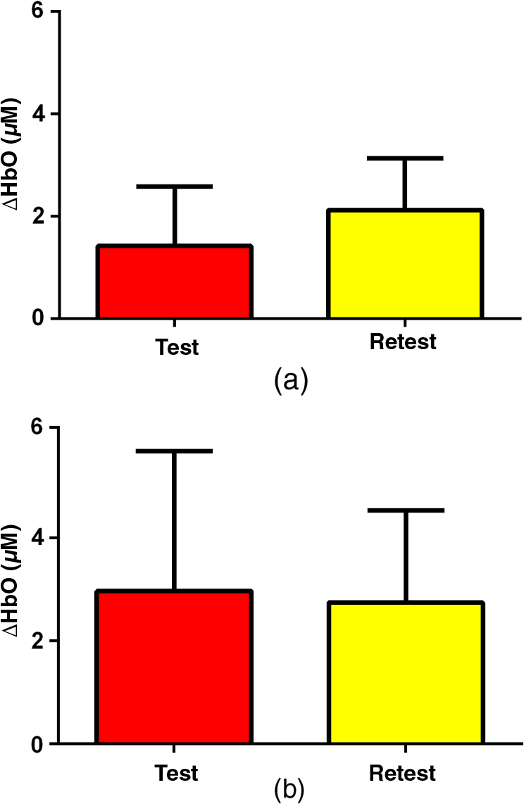
3.2.4.

Simple procedure for ICC selection

To provide convenience in practice for test-retest reliability assessment of neuroimaging measurements, the guidelines in Sec. 3.2.3 are summarized into a simple procedure for ICC selection considering general settings in neuroimaging studies. The flow chart of the procedure is shown in Fig. 1. The procedure consists of two steps. Step 1 is to determine if the test effect is negligible. At this step, the unified ANOVA model (i.e., two-way random-effect or two-way mixed-effect ANOVA model) would be constructed using the actual data. The significance of the between-tests variance is indicated by the $p$ value, which is often given as part of the ANOVA output. If it is not significant, it means that the test effect is negligible. Accordingly, the one-way random-effect model should be chosen, and ICC(1,1)/ICC(1, $k$ ) are the appropriate reliability measures. If the between-tests variance is significant, then the test effect is not negligible, and thus, two-way models should be used. Step 2 is to determine whether the test effect is random. Expert knowledge on the experimental system will be used to make the decision. If the systematic error is believed to be random, then the two-way random-effect model should be chosen, and ICC(2,1)/ICC(2, $k$ ) are appropriate reliability measures. If the researcher is not sure about the distribution of the systematic error or suspects a certain pattern to exist, then the two-way mixed-effect model should be chosen, and ICC(3,1)/ICC(3, $k$ ) are the appropriate reliability measures.

Fig. 1

Flow chart of the procedure for intraclass correlation coefficient (ICC) selection.

Two things need to be kept in mind when applying the above procedure for ICC selection in practice. (1) If the test effect is found to be negligible in step 1, the three models will yield similar ICC values, so any of them can be used in the reliability assessment of measurements as pointed out by guideline ii. The one-way model is suggested in the procedure because it is appropriate in the sense of model building. (2) Due to the subjectivity involved in the choice between the two-way random-effect versus mixed-effect model, the decision might be debatable in some cases. In fact, such debates widely exist among researchers in many other fields.¹^,² So finding an absolutely better model is not very meaningful here; the key is to make sure that the same model is grounded in comparing the reliability of neuroimaging modalities.

4. Assessment of Intertest Reliability on fNIRS-Based Brain Imaging Using ICC

To better illustrate the guidelines and interpret ICC analysis results, we apply the six forms of ICC to an actual research study in this section that uses fNIRS-based, volumetric diffuse optical tomography (vDOT) to image brain functions under a risk decision-making protocol.

4.1.

Measurements of BART-Stimulated vDOT

4.1.1.

Subjects, experimental setup, and study protocol

Nine healthy right-handed subjects (five males and four females, between 25 and 39 years) were recruited for this study. Written informed consent was obtained from all the subjects; the study protocol was approved by the University of Texas at Arlington institutional review board. All the subjects were scanned twice with a mean test-retest time interval of three weeks. No subjects reported any known diseases, such as musculoskeletal, neurological, visual, or cardiorespiratory dysfunctions. A continuous wave fNIRS brain imaging system (Cephalogics, Washington University, USA) was applied to each subject’s forehead to record the hemodynamic variation during risk decision-making tasks. Based on the modified Beer-Lambert law, two wavelengths (750 and 850 nm) were used to calculate changes of $Δ HbO$ and $Δ HbR$ . The fNIRS optode array consisted of 12 sources and 16 detectors with a nearest inter-optode distance of $\sim 3.25 cm$ , forming 40 measurement channels in total and covering the forehead entirely, as seen in Fig. 2. For more details on the instrumentation, see Ref. 23.

Fig. 2

(a) Optode locations coregistered to the ICBM152 brain template²⁴ and (b) the geometry of the probe, where circles represent the detectors and crosses represent the sources.

The study protocol was modified from the BART paradigm utilized in a previous fMRI study.²⁵ BART is a psychometrically well-established protocol, has predictive validity to real-world risk taking, and has been commonly used in the field of neuroscience as a behavioral measure to assess human risk-taking actions and tendencies while facing risks. A more detailed description of the computer-based BART paradigms can be found in Ref. 23. To briefly review it, the fNIRS-studied BART paradigm includes two outcomes or phases, that is, win and lose in response to wins (collect rewards) or losses (lose all rewards) during BART performances in both active and passive decision-making modes. For this test-retest reliability study, only the active mode was considered since the passive mode did not induce many significant changes in hemodynamic signals in the frontal cortex of each subject.²³ In each test, BART instructions were given first, and then the subjects played the computer-based BART tasks. A blocked-design was used; it consisted of a stimulation (i.e., balloon-pumping and/or decision-making process) period of 5 s and a recovery period of 15 s. A total of 15 blocks of tasks were assigned to each subject. Overall, it took 20 to 21 s to finish one block and $\sim 5$ to 6 min to complete an entire 15-balloon fNIRS-BART protocol. All the subjects were carefully instructed and performed short-test versions of the paradigms before the real task to allow familiarization with the devices and the protocols. To eliminate the environmental light contamination, the room was kept dark throughout the tasks. In addition, a black board was placed between the operating monitor and the optodes probe.

4.1.2.

Data processing for vDOT

The raw temporal data were first put into a band-pass filter (0.03 Hz for high-pass corner and 0.2 Hz for low-pass corner) to remove instrument drift and physiological noises.²⁶ Then a block-average process was performed on the data in order to enhance the signal-to-noise ratio. Here, we utilized a three-dimensional human head template (ICBM152) generated by T2-weighted MRI to develop a human brain atlas-guided finite-element model (FEM).²⁴ The forward modeling was subsequently conducted in the FEM and the sensitivity matrix was generated by using the FEM-based MATLAB® package, NIRFAST.²⁷ We applied a depth compensation algorithm (DCA) to the sensitivity matrix to compensate for the fast decay of sensitivity with the increase of depth.²⁸ Then the inverse modeling was conducted using Moore-Penrose generalized inversion with Tikhonov regularization.²⁹ The changes of absorption coefficient for each wavelength (750 and 850 nm) at each pixel were generated in this process. Values of ΔHbO, ΔHbR, and total hemoglobin concentration ( $Δ HbT$ )³⁰ from each voxel were computed by processing the fNIRS data from 0 to 5 s during the reaction/response phase right after the decision-making phase.²³ After combining DCA with DOT, we were able to form vDOT and to better estimate the detection depth up to $\sim 2.5$ to 3 cm below the scalp.³¹

To identify the activated areas and volumes in the cortex, the regions of interest (ROI) were defined or identified based on the reconstructed $Δ HbO$ values from the voxels within the field of view (FOV) by the $9 cm \times 20 cm$ optode-covered area (see Fig. 2). As mentioned above (Sec. 4.1.1), 12 sources and 16 detectors (with a nearest inter-optode distance of 3.25 cm) formed 40 measurement channels, which allowed us to form voxel-wise DOT with a detection layer up to 3 cm. Any voxel with a $Δ HbO$ value higher than a half of the maximum $Δ HbO$ determined over the FOV would be included or counted within the ROI. Namely, the ROIs were selected using the full-width-at-half-maximum (FWHM) approach based on a single maximum $Δ HbO$ value across both cortical sides of FOV. More details on ROI selection can be found in Ref. 23.

4.2.

Experimental Results of $Δ HbO$ -Based vDOT

4.2.1.

Hemodynamic response under BART stimulation

In our experimental study, the BART risk decision-making task was performed by the nine young healthy participants twice (visit 1 and visit 2). $Δ HbO$ values within the FOV were computed during a 5-s period of post decision-making reaction time for each visit. The activated pixels were extracted by the FWHM threshold. Figure 3 shows the reconstructed $Δ HbO$ maps of brain activations on the cortical surface with three different views: coronal (left), sagittal (middle), and axial (right). This figure clearly illustrates the brain activation areas in both visits for win (upper image) and lose (bottom image) cases. The group averaged activated pixels are highlighted as red (for visit 1) and yellow (for visit 2). All responses to BART from visit 1 and visit 2 robustly evoked hemodynamic signal increases in their respective anatomical regions. It was observed that both win and lose cases in the two visits revealed strong positive activations in both left and right dorsal-lateral prefrontal cortex (DLPFC) regions.

Fig. 3

Coronal, sagittal, and axial views of oxygenated hemoglobin changes ( $Δ HbO$ ) activation in volumetric diffuse optical tomography images at the group level from visit 1 (red), visit 2 (yellow), and their overlap (white). Upper images show reaction cortical regions/volumes under the win stimulus, while bottom images represent those under the lose stimulus.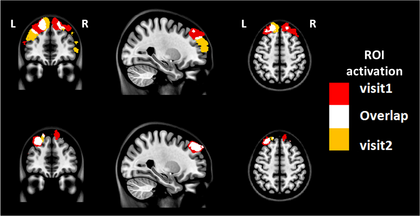

Specifically, there was a more focused or overlapped brain activation region (white areas) in the lose case (lower row of Fig. 3) than in the win case (upper row of Fig. 3) between both visits. Also, all brain images revealed a higher level and a larger area of left DLPFC activation than those in the right DLPFC region. These results, which are consistent with reported findings in the literature, suggest that specific neural regions (the lateral PFCs and dorsal anterior cingulate) support cognitive control over thoughts and behaviors, and that these regions could potentially contribute to adaptive and more risk-averse decision making.²³^,²⁵

To test the statistical differences between visit 1 and visit 2, a pairwise $t$ test was performed on the mean amplitude of ΔHbO in both win and lose cases; the results ( $mean \pm s . d .$ ) are shown in Fig. 4. No significant difference was found in both the win ( $1.42 \pm 0.39 μ M$ in visit 1 and $2.12 \pm 0.34 μ M$ in visit 2, $n = 9$ , $p$ $value = 0.19$ ) and lose case ( $2.97 \pm 0.90 μ M$ in visit 1 and $2.74 \pm 0.59 μ M$ in visit 2, $n = 9$ , $p$ $value = 0.84$ ). The results indicate that there was no significant difference between the two visits at the group-mean amplitude level.

Fig. 4

Bar plots of the mean $Δ HbO \pm standard deviation$ of the two visits in (a) win and (b) lose case.

4.2.2.

Reliability assessment using ICC

To assess the test-retest reliability of vDOT in the two cases (win and lose), we computed the six forms of ICC as defined in Table 5 using the mean ROI-based $Δ HbO$ values in Table 6. The values of the ICCs are presented in Table 7. Note that $k = 2$ in this study. It is observed that in the lose case, the ICCs of a single measurement and ICCs of the average measurement were relatively consistent, whereas those in the win case vary considerably and, thus, will lead to different conclusions. For example, if ICC(1,1) was used, we would conclude that the test-retest reliability was fair ( $0.4 < ICC < 0.6$ ), while if ICC(3,1) was used, a good reliability ( $0.6 < ICC < 0.75$ ) could be concluded (see Sec. 2.3). This clearly illustrates the necessity and importance of ICC selection as discussed in the Introduction.

Table 6

Region of interest–based mean ΔHbO at individual level.

Subject (ID)	Win (ΔHbO in μM)		Lose (ΔHbO in μM)
	Visit 1	Visit 2	Visit 1	Visit 2
1	1.04	3.27	1.74	0.68
2	4.15	3.95	5.06	4.86
3	2.36	2.25	6.58	5.62
4	1.09	1.36	1.56	3.80
5	0.64	1.59	7.68	2.28
6	0.92	1.02	0.92	0.58
7	0.70	1.08	0.44	1.34
8	0.45	1.87	1.20	2.30
9	1.39	2.69	1.58	3.24

Table 7

Intraclass correlation coefficients (95% confidence interval) for assessing test-retest reliability.

Task	ICC(1,1)	ICC(2,1)	ICC(3,1)	ICC(1,2)	ICC(2,2)	ICC(3,2)
Win	0.58(0,0.89)	0.61(0,0.90)	0.72(0.16,0.93)	0.73(0,0.94)	0.76(0,0.95)	0.84(0.27,0.96)
Lose	0.56(0,0.88)	0.54(0,0.88)	0.52(0,0.87)	0.71(0,0.93)	0.7(0,0.94)	0.68(0,0.93)

The appropriate ICCs in the two cases can be determined following the guidelines summarized in Sec. 3.2.3, as explained below.

Under guideline (i), since the experimental conditions for all subjects were the same in each visit, this rule does not apply here.

Under guideline (ii), to decide whether to choose the one-way model or two-way model, we conducted two-way ANOVA analysis to find the significance of between-tests variance. The resulting ANOVA tables in the win case and lose case are given in Tables 8 and 9, respectively. In the win case, the $p$ value of the $F$ test is 0.03, indicating that the between-tests variance is significant (assuming significance $level = 0.05$ ). The calculated magnitudes of the ICCs have the order of ICC(1,1) $< ICC (2,1)$ $< ICC (3,1)$ , which is consistent with property 2 given in Sec. 3.1. According to guideline (ii), the two-way model should be chosen in this case. In the lose case, the $p$ value is 0.77, indicating the insignificance of the between-tests variance. The magnitudes of the ICCs are close to each other, which is also consistent with property 2. By guideline (ii), ICCs based on any of the three models can be used in this case.

Table 8

ANOVA tablea in the win case.

Source	df	SS	MS	F	p value
Test	1	2.23	2.23	6.62	0.03
Subject	8	16.43	2.05	6.09	0.01
Residual	8	2.70	0.34
Total	17	21.37

Note: SS, sum of squares; MS, mean squares; MS=SS/df; F, statistic in the F test.

^aSummary of ANOVA results, which are standard output from software SAS.

Table 9

ANOVA table in the lose case.

Source	df	SS	MS	F	p value
Test	1	0.24	0.24	0.09	0.77
Subject	8	63.85	7.98	3.14	0.06
Residual	8	20.34	2.54
Total	17	84.43

Under guidelines (iii) and (iv), a further determination was needed on whether to choose the two-way random-effect model or mixed-effect model for the win case. First, we believe that the systematic error of our experimental system is random (assuming minimal learning effects in our study since the time interval between the two visits was long enough) and results in this study can be generalized to all possible tests on the system. Such a generalization is also desirable as the ultimate goal of our study is to test the general feasibility of vDOT as a brain imaging tool for assessing risk decision making. Second, we are concerned with the absolute agreement of measurements in the test-retest reliability analysis. By guideline (iii), ICCs based on the two-way random-effect model should be used.

In summary, ICC(2,1)/ICC(2,2) should be used in the win case, and any of the three types of ICCs, i.e., ICC(1,1)/ICC(1,2), ICC(2,1)/ICC(2,2), ICC(3,1)/ICC(3,2), could be used in the lose case. For convenience in practice, we prefer to use a single ICC protocol for reliability analysis. Thus, we conclude that ICC(2,1)/ICC(2,2) should be chosen in this study. Further, based on Table 7, we conclude that in the win case, (1) a single measurement has good reliability, while the average of test-retest measurements has excellent reliability; (2) in the lose case, a single measurement has fair reliability, while the average of test-retest measurements has good reliability. Note that in Table 7, ICCs of the average measurement are always larger than their counterparts of a single measurement, which is consistent with property 3 in Sec. 3.1.

4.3.

Relationship between Behavioral Reliability and vDOT Intertest Reliability

It is important to investigate the relationship between ICC values of behavioral measures and HbO measures by vDOT in order to correctly interpret the test-retest results. Table 10 shows corresponding test-retest ICCs from the behavioral data. It is seen that in the win case, the behavioral reliability assessed by ICC(1,1) and ICC(2,1) is fair, while that assessed by ICC(3,1), ICC(1,2), ICC(2,2), and ICC(3,2) is relatively high, i.e., good to excellent. In the lose case, however, the reliability assessed by ICC(1,1), ICC(2,1), and ICC(3,1) is poor, and that assessed by ICC(1,2), ICC(2,2), and ICC(3,2) is fair. These results indicate that the behavioral data are less stable than the vDOT measured data (see Table 7). However, after we investigated the correlation of ICC values of the behavioral data and the HbO data, we found high consistency of these two datasets. The correlations (quantified by Pearson’s correlation coefficient $R$ ) in the win and lose case are 0.96 and 0.99, respectively. To demonstrate this point, Fig. 5 shows the six types of ICC values for HbO and behavior score in the two cases.

Table 10

Intraclass correlation coefficients with 95% confidence interval for behavioral data.

Task	ICC(1,1)	ICC(2,1)	ICC(3,1)	ICC(1,2)	ICC(2,2)	ICC(3,2)
Win	0.54(0,0.87)	0.59(0,0.90)	0.77(0.28,0.94)	0.70(0,0.93)	0.74(0,0.95)	0.87(0.44,0.97)
Lose	0.37(0,0.81)	0.36(0,0.81)	0.36(0,0.81)	0.53(0,0.90)	0.53(0,0.89)	0.53(0,0.90)

Fig. 5

ICC values for HbO and behavior score in the win and lose cases.

5. Discussion

5.1.

Single Measurement versus Average of Repeated Measurements

As mentioned at the beginning of Sec. 3.2, the selection of ICCs is essentially based on the three ANOVA models. Once the model is chosen, either the ICC of a single measurement or that of the average measurement can be calculated for reliability assessment. Usually both of the metrics are used to quantify the reliability of measurements.⁵^,⁸^,⁹^,¹¹ This will provide important information on the effect of repeated testing on intertest reliability and will help make a decision on how many tests are needed. Taking the calculated ICC values in Table 7 as an example, $ICC (2,1) = 0.61$ and $ICC (2,2) = 0.76$ in the win case. This means that if the status of a subject is represented using a single measurement (that is, only one visit is done in the study), the reliability is 0.61; if it is represented using the average of the subject’s measurements in visit 1 and visit 2, the reliability is 0.76. In other words, adding a second visit can enhance the intertest reliability by 0.16. If a reliability of 0.61 is acceptable, then a single visit would be enough to measure the status of subjects; otherwise, two or more visits are needed.

5.2.

ICC Selection Through Statistical Model Comparison

The choice between the two-way random-effect model and mixed-effect model can also be made by comparing these two models through statistical model comparison methods. A popular simple method is to compare the Akaike information criterion (AIC) or Bayesian information criterion (BIC) of the models.³² AIC and BIC measure the performance of a statistical model in fitting a given dataset and attempt to achieve a trade-off between goodness-of-fit of the model and its complexity. A smaller value of these two measures indicates a better model. Due to a small sample size that is often the case in test-retest neuroimaging measurements, however, these statistical measures may not provide reliable results. Moreover, concerns from a statistical perspective (e.g., goodness-of-fit, model complexity, etc.) may not make much practical sense in reliability studies. To show the performance of the above method, AIC and BIC of the random-effect model and mixed-effect model were computed and are listed in Table 11. As shown in the table, the AIC/BIC of the two models are very similar in both the win and lose cases, meaning that the two measures do not provide sufficient evidence for model selection.

Table 11

Results of Akaike information criterion (AIC)/Bayesian information criterion (BIC) in the model selection.

	Two-way random ANOVA model		Two-way mixed ANOVA model
Task	AIC	BIC	AIC	BIC
Win	57	60.56	54.86	58.43
Lose	83.19	86.75	81.88	85.44

5.3.

Special Issues in Reporting and Interpreting ICCs

There are some special issues that may arise in assessing test-retest reliability of measurements using ICCs. The first issue is negative reliability estimates. Since ICCs are defined to be the proportion of between-subjects variance, they should theoretically range from 0 to 1. In practice, however, due to sampling uncertainty, the calculated values of ICCs may be out of the theoretical range, such as being negative. To be meaningful, negative ICC values can be replaced by 0 (e.g., Ref. 33). The second issue is dependence of ICCs on between-subjects variance. According to the definitions of ICC in Eqs. (6) and (7), the value of ICCs depends on the between-subjects variance. When the between-subjects variance is small, i.e., subjects differ little from each other, even if the measurement error variance is small, the ICC may still be small; on the other hand, large between-subjects variance may lead to large ICCs even if the measurement error variance is not small. For example, considering ICCs defined by Eq. (7), if between-subjects $variance = 0.2$ and random error $variance = 0.3$ , $ICC = 0.2 / (0.2 + 0.3) = 0.4$ ; if between-subjects $variance = 3$ and random error $variance = 1$ , $ICC = 3 / (3 + 1) = 0.75$ . Taking into account the magnitude of the between-subjects variance and random error variance, the former ( $ICC = 0.4$ ) might be acceptable, while the latter ( $ICC = 0.75$ ) might not be satisfactory in some applications. So the meaning of ICCs is context specific,³ and it is not adequate to compare the reliability in different studies only based on ICCs. The final issue is significant between-tests variance. When ANOVA indicates that the between-tests variance is significant, the value of ICCs may still be large, indicating good reliability. However, the significant between-tests variance is not desirable and efforts need to be made to reduce the systematic error of the test. For example, protocols of the study may be modified to eliminate the learning effects of the test.³⁴

5.4.

Consistency of ICCs between Behavioral and HbO Measurements

Figure 5 clearly demonstrates that in the win case, we had an excellent agreement of ICC values between HbO and behavior data. In the meantime, data in the lose case also show a consistent trend from ICCs of a single measurement to ICCs of the average measurement, which could be interpreted as that the reproducibility/reliability of hemodynamic measurements during the risk decision-making task has an improvement pattern consistent with the behavior score reliability. Furthermore, the poor-to-fair ICC scores in behavior reliability in the lose case may imply that parts of the nonreliability in the lose case may be attributable to the source of variable behaviors when the subjects faced the undesirable loss during risk-taking actions. Overall, these findings suggest that the amplitude of HbO is a suitable biomarker for risk decision-making studies. Further research is needed to identify other potential unstable sources that contribute to the variation in the test-retest repeatability of fNIRS-based measurements under risk decision-making tasks.

5.5.

Effects of Extra-Cranial Signals in Reliability Assessment

The broad range of fNIRS studies are always faced with the issue of extra-cranial signals that may cause errors in fNIRS measurements.³⁵^–³⁷ The first concern is the personal variation in scalp-to-cortex distance, which may confound fNIRS signals from cortical regions. Many groups have reported their investigations on extra-cranial-dependent fNIRS sensitivity. Recent studies indicate that the impact of scalp-to-cortex distance on the fNIRS exists and suggest including head circumference as a control factor on practical measurements.³⁷ A more careful study on reward tasks using combined fNIRS and fMRI reveals that the increase of sensitivity to reward and scalp-to-cortex distance decreases the correlation between fNIRS data and fMRI data.³⁵ Moreover, it is found that blood pressure fluctuations can also affect the fNIRS measurement in the superficial cortex.³⁶ The second concern is the variation in neural responses. A recent study in the fMRI field indicates that there may be more influence from physiological noises than the brain activation under emotion stimulus.³⁸

Nonetheless, in a test-retest reliability study, such concerns may not be essential. First, since we can safely assume that the anatomy within a subject was stable during the two-week test-retest period, the variation due to the first concern, i.e., scalp-to-cortex distance, could be ignored. Also, more advanced data processing methods can be developed and introduced to further minimize the effects of extra-cranial signals. For example, a recent study by performing an easy-to-use filter method on all fNIRS channels to subtract the extra-cranial signal shows substantial improvement in the forehead measurement.³⁹ In addition, a double short separation measurement approach based on the short-distance regression could also be introduced to reduce the extra-cranial noise for both HbO and HbR signals.⁴⁰

5.6.

Future Research

Future research should extend the study of reliability. The following are two topics that need to be investigated. First, neuroimaging data are often obtained from the commonly used modalities, such as fMRI, fNIRS, PET/SPECT, including information on both activation pattern and activation amplitude. This study examined amplitude agreement using ICCs. In order to fully assess the test-retest reliability of a neuroimaging measurement, the pattern reproducibility should also be examined.²² Dice coefficient for pattern overlap and Jaccard coefficient could be used for this purpose.⁴¹ Second, instead of using an ROI-averaged amplitude or significant cluster amplitude to quantify the ICCs, Caceres et al. proposed a map-wised ICCs approach, which conducts voxel-wise ICC analysis for the whole brain.⁴² This approach can help discriminate the best ROIs between individuals and correlate the ICC map with the activation map since both metrics were voxel-based. We will apply this approach to study the reliability of measurements in future research.

6. Conclusion

Choosing appropriate forms of ICC is critical in assessing intertest reliability of neuroimaging modalities. A wrong choice of ICCs will lead to misleading conclusions. In this study, we have reviewed the statistical rationale of ICCs and provided guidelines on how to select appropriate ICCs from the six popular forms of ICC. Also, based on $Δ HbO$ activation maps by fNIRS-based vDOT under a risk decision-making protocol, we have demonstrated appropriate ICC selections and assessed the test-retest reliability of vDOT-based brain imaging measurements following the given guidelines. While this study provides a statistical approach to assess test-retest reliability of fNIRS measurements, its understanding and guidelines of ICCs are applicable to other neuroimaging modalities. Better comprehension of ICCs will help neuroimaging researchers to choose appropriate ICC models, perform accurate reliability assessment of measurements, and make optimal experimental designs accordingly.

Acknowledgments

L. Li thanks Dr. Lorie Jacobs for her assistance and support for preparation of the manuscript. Authors also acknowledge two MATLAB^®-based packages available on the website, which are FEM solver NIRFAST: http://www.dartmouth.edu/~nir/nirfast/ and mesh generator iso2mesh: http://iso2mesh.sourceforge.net/cgi-bin/index.cgi.

References

1.

P. E. Shrout and J. L. Fleiss, “Intraclass correlations: uses in assessing rater reliability,” Psychol. Bull., 86 (2), 420 –428 (1979). http://dx.doi.org/10.1037/0033-2909.86.2.420 PSBUAI 0033-2909 Google Scholar

2.

K. O. McGraw and S. P. Wong, “Forming inferences about some intraclass correlation coefficients,” Psychol. Methods, 1 30 –46 (1996). http://dx.doi.org/10.1037/1082-989X.1.1.30 1082-989X Google Scholar

3.

J. P. Weir, “Quantifying test-retest reliability using the intraclass correlation coefficient and the SEM,” J. Strength Cond. Res., 19 231 –240 (2005). http://dx.doi.org/10.1519/15184.1 1064-8011 Google Scholar

4.

Y. Bhambhani et al., “Reliability of near-infrared spectroscopy measures of cerebral oxygenation and blood volume during handgrip exercise in nondisabled and traumatic brain-injured subjects,” J. Rehabil. Res. Dev., 43 (7), 845 (2006). http://dx.doi.org/10.1682/JRRD.2005.09.0151 JRRDEC 0748-7711 Google Scholar

5.

M. M. Plichta et al., “Event-related functional near-infrared spectroscopy (fNIRS): are the measurements reliable?,” Neuroimage, 31 (1), 116 –124 (2006). http://dx.doi.org/10.1016/j.neuroimage.2005.12.008 NEIMEF 1053-8119 Google Scholar

6.

U. Braun et al., “Test-retest reliability of resting-state connectivity network characteristics using fMRI and graph theoretical measures,” Neuroimage, 59 (2), 1404 –1412 (2012). http://dx.doi.org/10.1016/j.neuroimage.2011.08.044 NEIMEF 1053-8119 Google Scholar

7.

M. M. Plichta et al., “Event-related functional near-infrared spectroscopy (fNIRS) based on craniocerebral correlations: reproducibility of activation?,” Hum. Brain Mapp., 28 733 –741 (2007). http://dx.doi.org/10.1002/(ISSN)1097-0193 HBRME7 1065-9471 Google Scholar

8.

H. Zhang et al., “Test-retest assessment of independent component analysis-derived resting-state functional connectivity based on functional near-infrared spectroscopy,” Neuroimage, 55 (2), 607 –615 (2011). http://dx.doi.org/10.1016/j.neuroimage.2010.12.007 NEIMEF 1053-8119 Google Scholar

9.

J.-H. Wang et al., “Graph theoretical analysis of functional brain networks: test-retest evaluation on short- and long-term resting-state functional MRI data,” PLoS One, 6 (7), e21976 (2011). http://dx.doi.org/10.1371/journal.pone.0021976 1932-6203 Google Scholar

10.

M. M. Plichta et al., “Test-retest reliability of evoked BOLD signals from a cognitive-emotive fMRI test battery,” Neuroimage, 60 (3), 1746 –1758 (2012). http://dx.doi.org/10.1016/j.neuroimage.2012.01.129 NEIMEF 1053-8119 Google Scholar

11.

F. Tian et al., “Test-retest assessment of cortical activation induced by repetitive transcranial magnetic stimulation with brain atlas-guided optical topography,” J. Biomed. Opt., 17 (11), 116020 (2012). http://dx.doi.org/10.1117/1.JBO.17.11.116020 JBOPFO 1083-3668 Google Scholar

12.

C. C. Guo et al., “One-year test-retest reliability of intrinsic connectivity network fMRI in older adults,” Neuroimage, 61 (4), 1471 –1483 (2012). http://dx.doi.org/10.1016/j.neuroimage.2012.03.027 NEIMEF 1053-8119 Google Scholar

13.

H. Niu et al., “Test-retest reliability of graph metrics in functional brain networks: a resting-state fNIRS study,” PLoS One, 8 (9), e72425 (2013). http://dx.doi.org/10.1371/journal.pone.0072425 1932-6203 Google Scholar

14.

M. Fiecas et al., “Quantifying temporal correlations: a test-retest evaluation of functional connectivity in resting-state fMRI,” Neuroimage, 65 231 –241 (2013). http://dx.doi.org/10.1016/j.neuroimage.2012.09.052 NEIMEF 1053-8119 Google Scholar

15.

H. Cao et al., “Test-retest reliability of fMRI-based graph theoretical properties during working memory, emotion processing, and resting state,” Neuroimage, 84C 888 –900 (2013). http://dx.doi.org/10.1016/j.neuroimage.2013.09.013 NEIMEF 1053-8119 Google Scholar

16.

D. V. Cicchetti, “Guidelines, criteria, and rules of thumb for evaluating normed and standardized assessment instruments in psychology,” Psychol. Assess., 6 284 –290 (1994). http://dx.doi.org/10.1037/1040-3590.6.4.284 PYASEJ 1040-3590 Google Scholar

17.

J. L. Fleiss, The Design and Analysis of Clinical Experiments, John Wiley & Sons, Inc., Hoboken, NJ (1999). Google Scholar

18.

X.-H. Liao et al., “Functional brain hubs and their test-retest reliability: a multiband resting-state functional MRI study,” Neuroimage, 83 969 –982 (2013). http://dx.doi.org/10.1016/j.neuroimage.2013.07.058 NEIMEF 1053-8119 Google Scholar

19.

D. J. Brandt et al., “Test-retest reliability of fMRI brain activity during memory encoding,” Front. Psychiatry, 4 163 (2013). http://dx.doi.org/10.3389/fpsyt.2013.00163 1664-0640 Google Scholar

20.

T. J. Kimberley, G. Khandekar and M. Borich, “fMRI reliability in subjects with stroke,” Exp. Brain Res., 186 183 –190 (2008). http://dx.doi.org/10.1007/s00221-007-1221-8 EXBRAP 0014-4819 Google Scholar

21.

D. S. Manoach et al., “Test-retest reliability of a functional MRI working memory paradigm in normal and schizophrenic subjects,” Am. J. Psychiatry, 158 955 –958 (2001). http://dx.doi.org/10.1176/appi.ajp.158.6.955 AJPSAO 0002-953X Google Scholar

22.

C. M. Bennett and M. B. Miller, “How reliable are the results from functional magnetic resonance imaging?,” Ann. N. Y. Acad. Sci., 1191 133 –155 (2010). http://dx.doi.org/10.1111/nyas.2010.1191.issue-1 ANYAA9 0077-8923 Google Scholar

23.

M. Cazzell et al., “Comparison of neural correlates of risk decision making between genders: an exploratory fNIRS study of the Balloon Analogue Risk Task (BART),” NeuroImage, 62 1896 –1911 (2012). http://dx.doi.org/10.1016/j.neuroimage.2012.05.030 NEIMEF 1053-8119 Google Scholar

24.

J. L. Lancaster et al., “Bias between MNI and Talairach coordinates analyzed using the ICBM-152 brain template,” Hum. Brain Mapp., 28 (11), 1194 –1205 (2007). http://dx.doi.org/10.1002/(ISSN)1097-0193 HBRME7 1065-9471 Google Scholar

25.

H. Rao et al., “Neural correlates of voluntary and involuntary risk taking in the human brain: an fMRI study of the Balloon Analog Risk Task (BART),” Neuroimage, 42 (2), 902 –910 (2008). http://dx.doi.org/10.1016/j.neuroimage.2008.05.046 NEIMEF 1053-8119 Google Scholar

26.

A. Miyake et al., “How are visuospatial working memory, executive functioning, and spatial abilities related? A latent-variable analysis,” J. Exp. Psychol. Gen., 130 19 (2001). http://dx.doi.org/10.1037/0096-3445.130.4.621 JPGEDD 0096-3445 Google Scholar

27.

H. Dehghani et al., “Near infrared optical tomography using NIRFAST: algorithm for numerical model and image reconstruction,” Commun. Numer. Methods Eng., 25 711 –732 (2009). http://dx.doi.org/10.1002/cnm.v25:6 1069-8299 Google Scholar

28.

H. Niu et al., “Development of a compensation algorithm for accurate depth localization in diffuse optical tomography,” Opt. Lett., 35 (3), 429 –431 (2010). http://dx.doi.org/10.1364/OL.35.000429 OPLEDP 0146-9592 Google Scholar

29.

S. Arridge, “Optical tomography in medical imaging,” Inverse Probl., 15 (2), R41 –R93 (1999). http://dx.doi.org/10.1088/0266-5611/15/2/022 INPEEY 0266-5611 Google Scholar

30.

L. Kocsis, P. Herman and A. Eke, “The modified Beer-Lambert law revisited,” Phys. Med. Biol., 51 N91 –N98 (2006). http://dx.doi.org/10.1088/0031-9155/51/5/N02 PHMBA7 0031-9155 Google Scholar

31.

Z.-J. Lin et al., “Atlas-guided volumetric diffuse optical tomography enhanced by generalized linear model analysis to image risk decision-making responses in young adults,” Hum. Brain Mapp., 35 4249 –4266 (2014). http://dx.doi.org/10.1002/hbm.v35.8 HBRME7 1065-9471 Google Scholar

32.

M. H. Kutner et al., Applied Linear Statistical Models, 5th ed.McGraw Hill, New York (2005). Google Scholar

33.

T. A. Salthouse, “Aging associations: influence of speed on adult age differences in associative learning,” J. Exp. Psychol. Learn. Mem. Cogn., 20 1486 –1503 (1994). http://dx.doi.org/10.1037/0278-7393.20.6.1486 JEPCEA Google Scholar

34.

G. Atkinson and A. M. Nevill, “Statistical methods for assessing measurement error (reliability) in variables relevant to sports medicine,” Sports Med., 26 217 –238 (1998). http://dx.doi.org/10.2165/00007256-199826040-00002 SPMEE7 0112-1642 Google Scholar

35.

S. Heinzel et al., “Variability of (functional) hemodynamics as measured with simultaneous fNIRS and fMRI during intertemporal choice,” Neuroimage, 71 125 –134 (2013). http://dx.doi.org/10.1016/j.neuroimage.2012.12.074 NEIMEF 1053-8119 Google Scholar

36.

L. Minati et al., “Intra- and extra-cranial effects of transient blood pressure changes on brain near-infrared spectroscopy (NIRS) measurements,” J. Neurosci. Methods, 197 (2), 283 –288 (2011). http://dx.doi.org/10.1016/j.jneumeth.2011.02.029 JNMEDT 0165-0270 Google Scholar

37.

F. B. Haeussinger et al., “Simulation of near-infrared light absorption considering individual head and prefrontal cortex anatomy: implications for optical neuroimaging,” PLoS One, 6 (10), e26377 (2011). http://dx.doi.org/10.1371/journal.pone.0026377 1932-6203 Google Scholar

38.

I. Lipp et al., “Understanding the contribution of neural and physiological signal variation to the low repeatability of emotion-induced BOLD responses,” Neuroimage, 86 335 –342 (2014). http://dx.doi.org/10.1016/j.neuroimage.2013.10.015 NEIMEF 1053-8119 Google Scholar

39.

F. B. Haeussinger et al., “Reconstructing functional near-infrared spectroscopy (fNIRS) signals impaired by extra-cranial confounds: an easy-to-use filter method,” Neuroimage, 95 69 –79 (2014). http://dx.doi.org/10.1016/j.neuroimage.2014.02.035 NEIMEF 1053-8119 Google Scholar

40.

L. Gagnon et al., “Further improvement in reducing superficial contamination in NIRS using double short separation measurements,” Neuroimage, 85 (Pt 1), 127 –135 (2014). http://dx.doi.org/10.1016/j.neuroimage.2013.01.073 NEIMEF 1053-8119 Google Scholar

41.

N. J. Tustison and J. C. Gee, “Introducing Dice, Jaccard, and other label overlap measures to ITK,” Insight J., 1 –4 (2009). 1060-135X Google Scholar

42.

A. Caceres et al., “Measuring fMRI reliability with the intra-class correlation coefficient,” Neuroimage, 45 (3), 758 –768 (2009). http://dx.doi.org/10.1016/j.neuroimage.2008.12.035 NEIMEF 1053-8119 Google Scholar

Biography

Lin Li has been a graduate research assistant in the Department of Bioengineering at the University of Texas (UT) at Arlington and received his PhD in biomedical engineering from the Joint Graduate Program between UT Arlington and UT Southwestern Medical Center at Dallas. He received his BS degree from Huazhong University of Science and Technology in optoelectronic engineering. His research interest includes algorithm development and image processing for multimodal brain imaging and integrative neuroscience.

Li Zeng is an assistant professor in the Department of Industrial and Manufacturing Systems Engineering at UT, Arlington. She received her BS degree in precision instruments, MS degree in optical engineering from Tsinghua University, China, and PhD in industrial engineering and MS in statistics from the University of Wisconsin–Madison. Her research interests are process control in complex manufacturing and healthcare delivery systems and applied statistics.

Zi-Jing Lin is an assistant scientist at National Synchrotron Radiation Research Center (NSRRC), Taiwan. He received his MS degree in biomedical engineering from National Cheng Kung University, Taiwan and PhD degree in biomedical engineering from the Joint Graduate Program between the University of Texas (UT) at Arlington and UT Southwestern Medical Center at Dallas. His current research area focuses on algorithm development for biological image processing and Cryo-Soft-X-ray microscopy and tomography for cellular imaging.

Mary Cazzell is the director of Nursing Research and Evidence-Based Practice at Cook Children’s Medical Center in Fort Worth, Texas. She received her BS in nursing from Marquette University and PhD in nursing from UT at Arlington. Her research area focused on behavioral measurement of risk decision making and identification of related neural correlates, using optical imaging, across the lifespan.

Hanli Liu is a full professor of bioengineering at the UT, Arlington. She received her MS and PhD degrees from Wake Forest University in physics, followed by postdoctoral training at the University of Pennsylvania in tissue optics. Her current expertise lies in the field of near-infrared spectroscopy of tissues, optical sensing for cancer detection, and diffuse optical tomography for functional brain imaging, all of which are related to clinical applications.

Citation Download Citation

Lin Li, Li Zeng, Zi-Jing Lin, Mary Cazzell, and Hanli Liu "Tutorial on use of intraclass correlation coefficients for assessing intertest reliability and its application in functional near-infrared spectroscopy–based brain imaging," Journal of Biomedical Optics 20(5), 050801 (20 May 2015). https://doi.org/10.1117/1.JBO.20.5.050801

Published: 20 May 2015

Access the abstract

JOURNAL ARTICLE
13 PAGES

DOWNLOAD PAPER SAVE TO MY LIBRARY

GET CITATION

CITATIONS

Cited by 54 scholarly publications.

Explore citations on Lens.org

RIGHTS & PERMISSIONS

Get copyright permission Get copyright permission on Copyright Marketplace

KEYWORDS

Reliability

Neuroimaging

Brain

Functional magnetic resonance imaging

Data modeling

Statistical analysis

Brain imaging

1.

Introduction

Table 1

2.

Intraclass Correlation Coefficient

2.1.

Unified ANOVA Model

Table 2

Eq. (1)

Eq. (2)

Eq. (3)

Eq. (4)

Eq. (5)

2.2.

Six Forms of ICC

Table 3

Table 4

Eq. (6)

Eq. (7)

Table 5

2.3.

ICC Criteria to Assess Reliability of Measurements

3.

Selection of ICCs

3.1.

Properties of ICCs

3.2.

Guidelines on ICC Selection

3.2.1.

Determination of one-way model versus two-way model

3.2.2.

Determination of two-way random-effect model versus mixed-effect model

3.2.3.

General guidelines

3.2.4.

Simple procedure for ICC selection

Fig. 1

4.

Assessment of Intertest Reliability on fNIRS-Based Brain Imaging Using ICC

4.1.

Measurements of BART-Stimulated vDOT

4.1.1.

Subjects, experimental setup, and study protocol

Fig. 2

4.1.2.

Data processing for vDOT

4.2.

Experimental Results of ΔHbO-Based vDOT

4.2.1.

Hemodynamic response under BART stimulation

Fig. 3

Fig. 4

4.2.2.

Reliability assessment using ICC

Table 6

Table 7

Table 8

Table 9

4.3.

Relationship between Behavioral Reliability and vDOT Intertest Reliability

Table 10

Fig. 5

5.

Discussion

5.1.

Single Measurement versus Average of Repeated Measurements

5.2.

ICC Selection Through Statistical Model Comparison

Table 11

5.3.

Special Issues in Reporting and Interpreting ICCs

5.4.

Consistency of ICCs between Behavioral and HbO Measurements

5.5.

Effects of Extra-Cranial Signals in Reliability Assessment

5.6.

Future Research

6.

Conclusion

Acknowledgments

Experimental Results of $Δ HbO$ -Based vDOT