

|
|
1.IntroductionFunctional near-infrared spectroscopy (fNIRS) has seen an exponential development over the past 20 years with an impressive breadth of applications.1,2 One of the strong advantages of the technology as a functional brain imaging tool is its adaptability to challenging environments and populations, notably for developmental studies in infants and children,3 motor and gait studies in moving subjects,4–6 and the clinical translation of the modality to neurocritical care.7,8 While the modality is often cited as relatively tolerant to movements, especially in comparison to fMRI, the nature of these studies is prone to introduce motion artifacts (MAs) in the fNIRS data. Therefore, in parallel to hardware efforts to design instrumentation more resistant to motion,6,9,10 a recent body of work has focused on developing algorithms to detect and/or correct MAs. These approaches include adaptive, Wiener, and Kalman filtering,11,12 principal component analysis (PCA),13–15 spline interpolation,16 wavelet analysis,17,18 an approach using the expected negative correlation between oxy- and deoxyhemoglobin,19 and an autoregressive model.20 Diverse metrics have been proposed to quantify the contamination by MAs and to compare the performance of different motion correction techniques in order to identify the optimal one.15,20–23 Some studies have assessed the effect of MAs and of their correction directly on the raw signal, or on the concentration time traces, by computing the signal-to-noise ratio of the data.9,10,23 In previous studies, we and others instead used metrics related to the evoked hemodynamic response function (HRF) to brain activation,15,20–22 a largely reported measure in fNIRS studies. We compared different MA correction approaches based on how accurately and repeatedly they could retrieve the HRF despite the presence of motion. Cooper et al.21 added a synthetic HRF on real resting-state data acquired on stroke patients and contaminated by MAs. They showed that all motion correction approaches improved the recovery of the HRF compared to no correction and to simple rejection of the stimulus trials contaminated by MAs, with the best performing methods being wavelet filtering and spline interpolation. Similarly, Yücel et al.15 used resting-state data acquired on healthy subjects instructed to perform specific movements in order to intentionally introduce MAs, and subsequently added synthetic HRFs to the time series. We introduced a novel motion correction method, targeted PCA, which proved to be superior to other approaches in the studied datasets. In both these studies, the ground truth for the HRF was known as it had been added synthetically to the resting data contaminated by MAs. A different approach was used by Brigadoi et al., who analyzed real functional activation data contaminated by MAs, recorded during a speech study, and for which the true HRF was unknown. Instead of comparing the retrieved HRF to the ground truth, unknown in this case, the authors assessed the physiological plausibility of the retrieved HRF.22 Contrary to the studies of Cooper et al. and Yücel et al., where the MAs were uncorrelated to the onsets of the stimulus, the scenario studied by Brigadoi et al. was more challenging: the MAs arising from the subject talking occurred simultaneously to the stimulus onsets the subject was responding to. In agreement with Cooper et al., the authors showed that the motion correction was always preferable to trial rejection in this case. Further, they found the best approach for these real datasets to be wavelet filtering. In parallel to the traditional fNIRS studies based on evoked response to cerebral activation, a growing number of studies instead analyze the spontaneous oscillations in the fNIRS signal.24–35 These can be roughly divided into two categories: resting-state functional connectivity (rs-fc) studies24–28 and autoregulation and vascular reactivity studies.29–35 The first category observes neuronally driven oscillations that show correlations between functionally related regions, while the second category studies vascular oscillations driven by blood pressure or fluctuations. To our knowledge, no work has directly investigated the effect of MAs, and the optimal way to correct them, on these types of data. This is the question we address in the present study, by comparing resting-state data with minimal motion contamination, with added MAs, and after correction of these MAs. Under the broad term of fNIRS “oscillations” studies, the concept of HRF does not apply and there is no standard way to analyze the data. However, a commonly employed tool is the temporal correlation between two time traces. Functional connectivity maps are generally obtained by computing the correlation of the fNIRS signal between a seed channel and all other locations over the head.24,27,28 Autoregulation studies based on spontaneous oscillations analyze the data either in the temporal domain,29,33,34 or in the Fourier frequency domain with transfer function analysis.31,32,35,36 In the first case, metrics of interest are, for instance, the cross-correlation between NIRS and arterial blood pressure (ABP) or cerebral perfusion pressure (CPP),33,34 or between symmetrical NIRS channels.29 For instance, we observed in Muehlschlegel et al.29 a significantly reduced interhemispheric correlation (IHC) between symmetrical channels in severe stroke patients compared to a control group. Use of a wavelet-based correlation has also been proposed instead of the traditional correlation, to account for the fact that the measured physiological signals are not stationary.37 In the present study, we chose as our metric of interest the correlation between oxyhemoglobin fluctuations measured at rest on symmetrical channels bilaterally on the forehead. 2.Methods2.1.Subjects and Data CollectionNIRS data were collected in two distinct groups: 46 healthy adults and 36 stroke patients. Forty-six healthy volunteers with no history of cardiovascular or neurological disease were recruited at the University of Copenhagen, Denmark, and 36 patients with symptoms of stroke in the territory of the internal carotid artery were recruited from the Stroke Unit, Glostrup Hospital in Denmark. The Biomedical Research Ethics committee in the Capital Region of Denmark approved both studies (H-B-2008-039 and H-B-2008-088). All subjects gave informed consent to participate in the study, which was undertaken in accordance with the Helsinki Declaration of 1964, as revised in Edinburgh in 2000. Subsets of this data have been previously analyzed and published independently.21,30,38 The NIRS data were collected with a TechEn Inc. (Milford, Massachusetts) CW6 system. NIRS optodes were placed bilaterally and symmetrically on the forehead, with, on each side, one source (690 and 830 nm) and one detector 3 cm away, avoiding the midline sinus. Additional channels were recorded at other locations in the two groups, but were not analyzed for the present study. NIRS recordings were acquired at a sampling rate of 200 Hz and were subsequently downsampled to 25 Hz. Each dataset consisted of 10 min of resting-state NIRS recording. Both the healthy subjects and stroke patients were placed in a supine position in a silent room with a constant temperature and the light dimmed. After 15 min of rest in the supine position, a 10-min trial of spontaneous breathing was acquired. 2.2.Data Analysis: Interhemispheric CorrelationFor each channel, the raw intensities at 690 and 830 nm were converted to relative changes in optical density using the modified Beer–Lambert law with a differential path length factor of 6 at both wavelengths. When applicable, MAs were identified and corrected on the time traces as detailed in Sec. 2.3. Then the corrected time series were converted to changes in oxy and deoxyhemoglobin concentrations, and , respectively. The hemoglobin concentration time series were band-pass filtered (third-order Butterworth low-pass filter and fifth-order Butterworth high-pass filter) in four different frequency bands of physiological interest: cardiac (0.5 to 1.5 Hz), respiration (0.15 to 0.5 Hz), low-frequency oscillations (LFOs, 0.05 to 0.15 Hz), and very LFOs (VLFO, 0.01 to 0.07 Hz). Finally, our metric of interest was the IHC between the two symmetrical channels on the forehead. Specifically, the IHC was computed as the correlation coefficient over the whole 10 min recording duration between the filtered time series of the two symmetrical channels on the forehead for each of the four frequency bands. Therefore, for each subject’s 10 min recording, we obtained four IHC values corresponding to the four physiological frequencies. The IHC values are between and , with meaning that the symmetrical channels are perfectly in phase, representing perfect anticorrelation (180-deg phase), and 0 representing either a complete lack of correlation between the channels or a 90-deg phase shift. 2.3.Motion Artifact Identification and CorrectionMAs were detected on the time series using the function hmrMotionArtifactPerChannel from the Homer2 processing package,39,40 except for the wavelet motion correction procedure, which performs the MA identification as part of the correction analysis. For each data channel, the algorithm automatically identifies MAs based on fast changes in signal amplitude and/or standard deviation. If, over a temporal window of length tMotion, the standard deviation increases by a factor exceeding SDThresh, or the peak-to-peak amplitude exceeds AMPThresh, then the segment of data of length tMask starting at the beginning of that window is defined as motion. We used , , , and for all datasets. In practice, these parameters may be tweaked on an individual-subject or -study basis in order to optimize the MA identification as confirmed by visual inspection. In the present study, in order to perform an objective characterization of MA incidence and of their correction, we fixed these parameters at the same values for all datasets in both groups. We compared five different MA correction approaches, which are illustrated in Fig. 1, left: not correcting the MAs (“No correction”), discarding the MA segments (“Discard”), spline interpolation correction (“Spline”),16 recursive-targeted PCA correction (“tPCA”),15 and wavelet filtering (“Wavelet”).18 The last three MA correction methods have been fully described by their respective authors and have been summarized in previous publications,15,21,22 so we only give a brief overview of the different algorithms here. Fig. 1Example illustrating: (a) a motion-free segment of data, (b) the same data after addition of MA segments, which are identified by the gray areas, and the different motion correction procedures: (c) discarding the MA segments, (d) spline interpolation, (e) targeted PCA, and (f) wavelet filtering. Left: at 830 nm for the symmetrical forehead channels. Right: time series for the symmetrical channels, after filtering in the LFO frequency band (0.05 to 0.15 Hz). The displayed IHC was computed over the whole 600 s of recording, but only 160 s of data are shown for better visualization of the MAs. 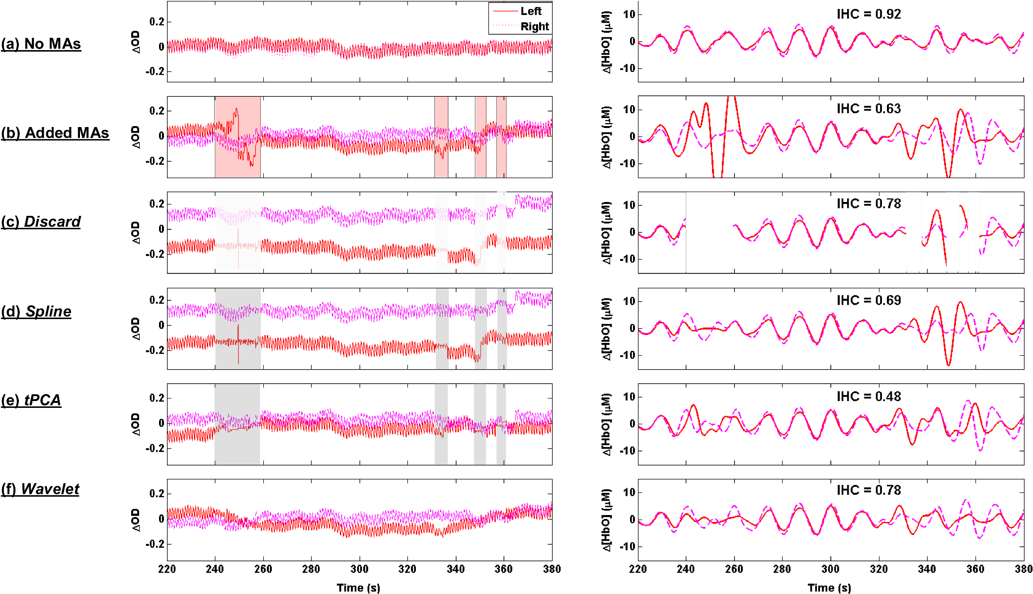 2.3.1.Motion artifact segment removal (discard)The simplest MA correction consisted in discarding all MA segments [Fig. 1(c)], i.e., computing the IHC on MA-free segments only. If an MA segment was identified in any of the four channels (two source-detector pairs at two wavelengths each), the time segment was ignored from the data in all channels. However, care must be taken in the management of the “ignored” MA-contaminated segments, so that they do not corrupt the adjacent MA-free segment through the subsequent step of band-pass filtering the data. Therefore, we first reconstruct the data in the MA segments using spline interpolation (as described below in Sec. 2.3.2), we then band-pass filter the data, and finally compute the IHC only on the time points originally identified as MA-free, as illustrated on Fig. 1(c), right. A more thorough discussion of this approach and a parallel with methods developed by Power et al.41,42 for fMRI data is presented in Sec. 4.2. 2.3.2.Spline interpolationWe applied the spline interpolation approach proposed by Scholkmann et al.,16 and incorporated in Homer2 as the hmrMotionCorrectSpline function [see Fig. 1(d)]. Each MA segment is first modeled with a cubic spline interpolation using the MATLAB® function csaps, and the modeled data are then subtracted from that segment of data. The successive corrected segments are then shifted by an offset that corresponds to the difference between the mean of the signal at the beginning of the MA segment and the mean of the signal at the end of the previous MA-free segment, following the framework detailed in Scholkmann et al.16 The smoothing parameter was set to 0.4, 0.9, and 0.99 successively. 2.3.3.Targeted principal component analysisWe applied the recursive-targeted PCA approach described in Yücel et al.,15 and integrated in Homer2 as the hmrMotionCorrectPCArecurse function [see Fig. 1(e)]. It consists of a recursive PCA method applied only to the segments identified as MAs rather than to the whole time series. At each iteration, the MAs are automatically identified using the procedure described in Sec. 2.3. If an MA is identified on one channel, then the segment is considered MA on all channels. The MA segments are then combined into a single matrix of size “number of MA time points” by “number of channels.” The PCA analysis converts the matrix of MA data into a set of orthogonal vectors (principal components), ranked in decreasing order of their contribution to the variance of the data. A certain number of principle components, accounting for a specific percent of the variance of the data they explain, is removed from the orthogonal matrix which is then transformed back into the corrected data. The segments of corrected motion are then stitched back into the original data time series by shifting the mean value of adjacent epochs of motion and motion-free data, following the same procedure used in the spline method above.16 The procedure of motion identification and correction is repeated for a total of iterations to remove any residual MAs. In this study, we used and set to 90%, 95%, and 97% successively. 2.3.4.Wavelet filteringWe used the discrete wavelet filtering approach described by Molavi and Dumont18 and incorporated in Homer2 as the hmrMotionCorrectWavelet function [see Fig. 1(f)]. Note that, for this approach, the MAs are both identified and corrected through the wavelet analysis so that we do not use the segments previously identified with Homer2. The time course is first decomposed in the wavelet domain using the general discrete wavelet transformation. The model assumes that the wavelet coefficients have a Gaussian probability distribution: the physiological components are centered around zero while MAs appear as outliers. The coefficients that are outside times the interquartile range (IQR) of the distribution are considered to represent MAs and are set to 0 before reconstructing the signal with the inverse discrete wavelet transform. The tuning parameter was set to 0.1, 0.8, and 1.5 in this work. 2.4.Motion Artifact AdditionA subset of the healthy datasets was used as reference data with minimal motion contamination. We selected all healthy datasets for which the cumulative duration of MA segments was less than 5% of the total recording time (34 datasets). On these “motion-free” datasets, we added MA segments obtained from the stroke datasets. 2.4.1.Same motion artifact content as the stroke groupFor each healthy recording, we randomly chose 20 stroke recordings from which to extract the MA segments, yielding a total of 680 datasets with added MAs. For each recording, the procedure to add MA segments, illustrated in detail in Fig. 2, was the following: one clean healthy dataset with no MA [Fig. 2(a)] was matched with a MA-contaminated stroke dataset [Fig. 2(b)]. The MA segments were identified on the stroke time series [Fig. 2(b)] as described in Sec. 2.3. Then the MA segments from the stroke time series were substituted in the healthy [Fig. 2(c)] on a per-channel and per-wavelength basis. Importantly, each MA segment was shifted in the healthy data by the same offset it was shifted in the stroke data. This shift can, for instance, be observed around on Figs. 2(b) and 2(c). An additional example of the procedure was provided in Figs. 1(a) and 1(b). The procedure was then repeated for all 20 selected stroke recordings. Fig. 2Illustration of the addition of motion artifacts (MAs) to healthy datasets: (a) The original time series from a healthy subject, with no identified MA. (b) The MA segments are identified on the time series of a stroke patient. (c) The MA segments are substituted in the healthy time series. The process is performed per source-detector pair and per wavelength. Only one channel is shown here (left side, 830 nm). The data offsets resulting from the MAs are also incorporated in the modified data. See for instance around , the baseline has been shifted negatively by about 0.2 after the MA segment to reflect the actual effect of the motion observed in the stroke dataset.  2.4.2.Larger motion artifact content than the stroke groupIn addition to the previous procedure where we artificially introduced the same MA content as that of the stroke datasets, we studied the effect of introducing further MA contamination. For this procedure, we first created a “pool” of 355 MA segments extracted from the stroke datasets as described above. Each MA consisted of the four segments of at the two wavelengths and the two channels. For each healthy dataset, we then added MA segments randomly selected from this pool at randomly selected time points, following the same segment substitution as described above (Sec. 2.4.1), in order to obtain a target average MA contamination. For each healthy dataset, we created 20 instances of randomly placed MA segments for the target MA contamination level. Finally, the whole process was repeated for different MA contamination levels varying from 17% up to 50% (duration of the cumulated MA segments over total recording duration). Figure 3 shows an example of a time series from the healthy dataset after introduction of a motion segment that results in approximately 10%, 30%, and 50% MA content. Note that this procedure results in a large number of short MAs as opposed to few long segments of MAs, so that the contamination higher than 50% corresponds to unusable datasets. Fig. 3Illustration of the addition of different levels of motion contamination to healthy data. The original time series from a healthy subject (blue) is contaminated by substitution of MA segments obtained from the stroke datasets, resulting in cumulative duration of MAs of 10%, 29%, and 52% (cyan).  2.5.Statistical AnalysisThe distribution of the number of MA segments is not Gaussian, and the distribution of IHC is bounded between and and is non-Gaussian. We, therefore, report the median and IQR of the number of MA segments and of the IHC values in the four frequency bands of interest for each group. To quantify the dependence of IHC on the number of MAs, we computed the Pearson correlation coefficient between the number of MAs and the Fisher’s Z-transform of the IHC. The Fisher Z-transformation normalizes the distribution of the IHC. We compared the IHC values between the following datasets: healthy without MA versus healthy with added MAs; healthy without MA versus healthy with added MAs, after MA correction; stroke versus healthy without MA; and stroke versus healthy with added MAs, before and after MA correction in both groups. To compare the IHC values between two datasets, we performed a two-sample Student -test applied on the Fisher Z-transformation of the IHC. Note that we report the median and IQR of the IHC before transformation for convenience, but all statistical analyses were performed on the Fisher Z-transform of the IHC. The threshold for significance was set to . 2.6.Overall MethodIn summary, our approach was the following. First, in Sec. 3.1, we study the correlation between incidence of MAs, and IHC, on the original (i.e., not MA-corrected) healthy and stroke datasets. Second, in Sec. 3.2, using only the healthy datasets with minimal MA contamination, we investigate the effect on IHC of adding MAs and of correcting them with the different approaches. We study in detail the case where synthetic motion contamination is equivalent to that of the stroke group, and further investigate how the different MA correction approaches perform when the MA contamination increases to up to 50% of the total recording time. This section provides a case where the ground truth IHC is known, and we can directly study the effect of MAs and their correction. Finally, in Sec. 3.3, we compare the healthy group after the addition of MA and the stroke group, in both cases with or without MA correction. The objective of this last part is to compare the healthy and stroke groups with similar MA contamination so as to minimize the confounding effect of motion contamination. 3.ResultsTable 1 presents the median and IQR of the IHC in the four frequency bands for the two groups (healthy and stroke) and for the different motion addition and correction approaches. Table 1Interhemispheric correlation (IHC) for the different groups and analyses in the four frequency bands of physiological interest. N is the number of subjects in the group. We report the median IHC and the interquartile range (IQR) in parentheses.
3.1.Interhemispheric Correlation Correlates with the Number of MAsAs illustrated in Fig. 4(a), without MA correction, the IHC (median and IQR) was significantly higher in the healthy group than in the stroke group at all frequencies: cardiac (healthy: 0.98, 0.95 to 0.99; stroke: 0.93, 0.84 to 0.96; ), respiration (healthy: 0.78, 0.55 to 0.90; stroke: 0.55, 0.22 to 0.76; ), low-frequency (healthy: 0.78, 0.66 to 0.89; stroke: 0.52, 0.01 to 0.68; ), and very-low frequency (healthy: 0.78, 0.64 to 0.90; stroke: 0.57, 0.41 to 0.71; ). The IQR values show that the variability across subjects was higher in the stroke group than in the healthy group in all frequency bands [see also error bars on Fig. 4(a)]. Fig. 4(a) IHC in the healthy group and the stroke group obtained with the original datasets (i.e., without MA addition or correction), in the four frequency band of interest. The colored circle represents the median and the error bars the IQR over all subjects. (b) Number of MA segments in the healthy group and the stroke group, obtained from the original datasets (median and IQR). For (a) and (b), the significance of the difference between the two group is displayed as * and **. (c) Scatter plot of the Fisher’s Z-transform of the IHC versus the number of MAs for the healthy subjects and the stroke patients. The displayed Pearson correlation coefficient and corresponding -value were computed over the combined data (healthy and stroke).  The number of MA segments was significantly lower () in the healthy group ( and to 5) than in the stroke group ( and to 13), as displayed in Fig. 4(b). Figure 4(c) shows the scatter plot, combined for both healthy and stroke groups, of the IHC in the low-frequency band versus the number of MAs. There is a significant negative correlation between the number of MAs and the IHC value (Pearson correlation coefficient: , ). The correlation was also significant in the cardiac (, ), and respiration (, ) frequency bands, and marginally significant in the VLFO (, ) frequency band. 3.2.Adding Motion Artifacts to Motion Artifact-Free Datasets Significantly Reduces Interhemispheric CorrelationThirty-four healthy datasets were considered motion-free as defined by the total duration of MA segments being under 5% of the total recording time (i.e., under 30 s over 10 min of recording). On this subset of data, the median (IQR) IHC was 0.98 (0.95 to 0.99), 0.85 (0.65 to 0.91), 0.80 (0.71 to 0.91), and 0.81 (0.66 to 0.90) in the cardiac, respiratory, LFO, and VLFO frequency bands, respectively. As expected from the results above, these values are slightly higher than the median values for the complete healthy group. After the addition of MAs on the healthy data subset, the IHC decreased significantly to 0.88 (0.77 to 0.95), 0.49 (0.23 to 0.73), 0.56 (0.34 to 0.74), and 0.60 (0.35 to 0.79) at the cardiac, respiration, LFO, and VLFO frequencies, respectively. This is significantly lower than the original values, with a -value of , , , and , respectively. This result is illustrated in Fig. 5 by the dark blue and cyan bars. As can be observed from the IQR values and from the error bars on Fig. 5, the addition of MAs also increased the variability of the IHC across subjects. Fig. 5Bar graph of the IHC in the healthy datasets with less than 5% MA contamination (blue), after addition of MA segments (cyan), and after motion correction using the discard method (gray), spline interpolation (green), targeted PCA (yellow), and wavelet analysis (magenta). The bar height represents the median, and the error bar the IQR over all subjects.  3.3.Effects of Different Motion Correction ApproachesWe performed a sensitivity analysis on the input parameters , , and for the Spline, tPCA, and Wavelet approaches, respectively. For each correction method, we assigned three values to the input parameters as described in Sec. 2. Working with the healthy dataset, we selected the value of each parameter that resulted in the least difference between the original IHC (on the MA-free datasets) and the IHC after MA addition and correction. This resulted in , , and . These values were employed in all subsequent results below. Figure 1 shows an example of the effect of the MA addition and correction on a short segment of motion-free healthy data. The first column displays the time traces at 830 nm of the two symmetrical channels, while the second column displays the corresponding times series after filtering in the 0.05 to 0.15 Hz frequency band. Figure 5 shows the effect of the different motion correction methods in the four frequency bands of interest for the healthy datasets with added MAs. All approaches increased the median IHC compared to the dataset with added MAs. However, all of them retrieved a value lower than the true IHC. Indeed, the IHC remained significantly lower than their original true values for all correction approaches. The performance of the different approaches differed. The discard approach performed best in all frequency bands, increasing the IHC to 0.95 (0.91 to 0.98) in the cardiac frequency band, 0.72 (0.50 to 0.85) in the respiration frequency band, 0.71 (0.56 to 0.81) in the LFO band, and 0.69 (0.51 to 0.79) in the VLFO band. The spline method increased the IHC to 0.91 (0.84 to 0.95) in the cardiac frequency band, 0.62 (0.38 to 0.78) in the respiration frequency band, 0.66 (0.48 to 0.77) in the LFO band, and 0.66 (0.50 to 0.78) in the VLFO band. Targeted PCA retrieved an IHC of 0.91 (0.82 to 0.96) in the cardiac frequency band, 0.57 (0.32 to 0.78) in the respiration frequency band, 0.61 (0.38 to 0.78) in the LFO band, and 0.63 (0.41 to 0.80) in the VLFO band. Finally, the wavelet analysis increased the IHC to 0.92 (0.86 to 0.96) in the cardiac frequency band, 0.71 (0.52 to 0.82) in the respiration frequency band, 0.65 (0.49 to 0.75) in the LFO band, and 0.62 (0.40 to 0.79) in the VLFO band. 3.4.Effect of Higher Motion Artifact ContentFigure 6 shows the evolution of the IHC, without MA correction and for the different MA correction approaches, as a function of the added MA content. The IHC decreases with increased MA content up to approximately 45% MA contamination. For higher MA content, the IHC starts to increase sharply. All MA correction methods improve the IHC, with the exception of the tPCA approach which degrades the IHC for MA content higher than . The discard approach performs best at all MA contents, and wavelet and spline have similar performances. However, even after MA correction, the IHC decreases for increasing MA contamination. Fig. 6IHC in the healthy datasets with less than 5% MA contamination after added MA, versus level of added MA contamination (expressed as percent of the total recording time). The results are presented after addition of MA segments (cyan), and after motion correction using the discard method (gray), spline interpolation (green), targeted PCA (yellow), and wavelet analysis (magenta). The blue and red arrows indicate the level of MA contamination corresponding to the original healthy datasets (no MA added) and to the original stroke datasets. 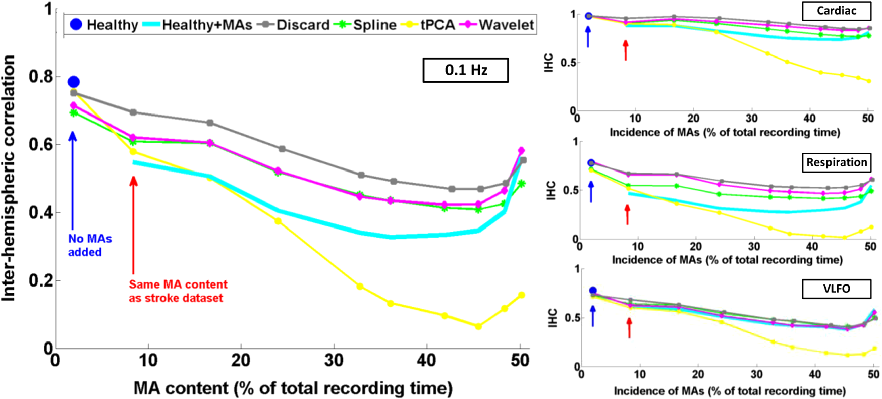 3.5.Comparison of Healthy with Added Motion Artifacts, and StrokeFigure 7 shows the effect of the different motion correction methods in the four frequency bands of interest for the stroke datasets. After the Discard motion correction, the median (IQR) IHC in the stroke group increased to 0.97 (0.93 to 0.98) at the cardiac frequency, 0.70 (0.51 to 0.77) at the respiration frequency, and decreased to 0.48 (0.34 to 0.66) in the LFO frequency band, and to 0.50 (0.34 to 0.62) in the VLFO frequency band. The spline procedure increased the IHC to 0.94 (0.88 to 0.96) at the cardiac frequency and 0.57 (0.42 to 0.71) at the respiration frequency, and decreased it to 0.46 (0.27 to 0.64) in the LFO frequency band, and 0.47 (0.29 to 0.61) in the VLFO frequency band. tPCA increased the IHC to 0.94 (0.82 to 0.97) at the cardiac frequency, and 0.62 (0.24 to 0.75) at the respiration frequency, and decreased it to 0.49 (0.27 to 0.67) in the LFO frequency band, and 0.55 (0.47 to 0.75) in the VLFO frequency band. Finally, the wavelet filtering increased the IHC to 0.96 (0.91 to 0.97) at the cardiac frequency, and 0.67 (0.47 to 0.76) at the respiration frequency, and had little effect in the lower frequency bands, where it retrieved 0.50 (0.30 to 0.67) in the LFO frequency band, and 0.57 (0.42 to 0.72) in the VLFO frequency band. Fig. 7Bar graph of the IHC in the stroke datasets (red), and after motion correction using the discard method (gray), spline interpolation (green), targeted PCA (yellow), and wavelet analysis (magenta). The bar height represents the median and the error bars the IQR over all subjects.  The IHC after MA addition in the healthy dataset was not significantly different than the IHC in the stroke group, in the respiration (), LFO (), and VLFO () frequency bands. At the cardiac frequency, the IHC was marginally lower in the healthy dataset with added MA than in the stroke dataset (). These results are illustrated in Fig. 8. Fig. 8Comparison of the IHC in the healthy group and the stroke group. The original healthy datasets (i.e., before MA addition, in dark blue) present high IHC in all frequency bands. After addition of MA segments obtained from the stroke dataset, the IHC in the healthy group (cyan) is significantly reduced at all frequencies and is not significantly different from the stroke IHC (red). After applying the discard procedure to these datasets (healthy with added MAs and stroke), the IHC is significantly lower in the stroke group than in the healthy group in the LFO frequency band, and marginally lower in the VLFO frequency band. Significance of the difference between the healthy and stroke datasets: (o) not significant (i.e., ), *, **.  Figure 8 also illustrates the comparison between the healthy group (without MA and with added MAs), and the stroke group, before and after the discard correction. After the discard motion correction, the IHC in the stroke group and in the healthy group with added MAs were not significantly different in the cardiac () and respiration () frequency bands. The IHC was significantly lower in the stroke group for the LFO (), and for the VLFO () frequency bands. We are not showing the comparison between the stroke and healthy groups for the other motion correction approaches, as they performed worse than discard in retrieving the “true” IHC in the healthy datasets, as detailed in Sec. 3.3. 4.Discussion4.1.Negative Correlation of Interhemispheric Correlation and Number of Motion ArtifactsWe observed that the IHC at all frequencies in the original datasets had a negative correlation with the number of MAs (results only shown for the LFO frequency band). Furthermore, adding MA segments to the healthy datasets with minimal MA contamination resulted in a significantly reduced IHC at all frequencies and in an increased IHC variability across subjects. The reduction of IHC with increased MA content can be counter-intuitive. If we assume motion to induce similar artifacts on all channels, we would expect the correlation between symmetrical channels to increase artificially with the presence of MAs. This effect was sometimes observed (data not shown). However, in most cases, the fast signal changes due to MA occur in opposite directions in different channels or with a slight delay, inducing a decrease in the IHC, as can be clearly observed in Fig. 1(b). See, for instance, in Fig. 1(b), right, around , an MA is present on both channels, resulting in an increase of the [HbO] fluctuations, albeit with a short delay between the two channels, which reduces IHC. The combination of these two effects results in an overall decrease of the IHC, but with increased variance. Note, however, that for very high MA content, the IHC starts to increase again, as illustrated in Fig. 7 for MA content . The very high number of synthetically incorporated MA segments is inducing correlations between channels. Due to the nature of the MA contamination we model here, which is typically a large number of short (a few seconds) motion segments, 50% MA contamination represents extremely “noisy” datasets (one out of two data points identified as motion-corrupted), which would be considered unusable in practice. Similar observations have been made in rs-fc blood oxygenation level-dependent fMRI studies. Power et al.41,42 reported that the motion affected correlation patterns over the brain, even when compensatory spatial registration and regression of motion estimates from the data were employed. They also observed that, while MAs tend to induce spurious increased correlations, some long-distance correlations were instead decreased by subject motion.41 Here, we observe an overall decrease in symmetrical forehead correlation with increased subject motion, but accompanied by increased variance, revealing that the IHC increased in some subjects and decreased in others. The contamination by MAs is an important confounding factor to take into account when interpreting NIRS data analysis based on correlations, as is mostly the case for oscillation-type studies such as functional connectivity and autoregulation studies. It is particularly crucial to be aware of this effect when comparing different populations, or different paradigms, that are prone to different levels of motion contamination. In the study presented here, the analysis of the original datasets revealed a highly significantly lower IHC in the stroke group compared to the healthy group at all frequencies. However, the number of MAs was also significantly higher in the stroke group, due to the difficulty for this clinical population to keep their head still during the whole duration of the recording. This suggested that the lower IHC in the stroke group was at least partly due to the higher MA content. Indeed, when adding motion segments identified on the stroke group to the healthy datasets, the IHC decreased to the level of the stroke group. In general, studies comparing a clinical population to a control healthy group might be subject to the same confounding effect of different motion contaminations. This possible confound should also be taken into account when studying the dependence of oscillations or functional connectivity on functional activity.43 A functional paradigm involving a motor or speech task could induce more MAs than the resting condition. Based on the present work, we, therefore, recommend that every study using correlation-based metrics and making comparisons between subjects or over time should test for MA content. 4.2.Implementation of the Discard ApproachThe implementation of the discard approach requires some care in the data analysis streamline. This is because the band-pass filtering step can spread artifacts due to motion from MA-contaminated segments onto the adjacent MA-free segments. If the band-pass filtering was performed before the removal of the MA segments, the large signal changes due to MAs would spread into the adjacent good MA segments through the filtering process. However, if instead the MA segments were first removed and the remaining good segments concatenated, this would also artificially modify the frequency content of the time series. Similarly, if the MA-free segments were zero-padded, spurious frequency content would artificially arise at each transition between MA-free and MA-contaminated segments replaced with zeros. Instead we first identify the MA segments and correct them using the spline interpolation approach in order to minimize any large change in signal. We then apply the band-pass filtering, and finally compute the IHC only on the segments originally identified as motion free. This same issue has already been recognized for the correction of MAs in rs-fc fMRI data and has been recently thoroughly discussed by Power et al.41,42 They proposed the following approach for fMRI resting state data analysis: first the “bad” data points contaminated by MAs are identified using objective data quality metrics, then the data points of these MA segments (the censored “bad” time points) are reconstituted using the MA-free segments (the uncensored “good” data), using a least-square spectral decomposition adapted for nonuniformly sampled data.44 Next, the reconstituted signal is band-pass filtered. Following the frequency-filtering, the reconstituted and filtered signals are “recensored,” i.e., the data points corresponding to the originally identified MA segments are ignored. Power et al.42 refer to this procedure as “scrubbing” the data. We implement a similar approach here, but we reconstitute the signal using the spline interpolation instead of the least square spectral decomposition. The rationale is identical: we implement a motion correction routine on the MA-contaminated segments prior to band-pass filtering, because, even though these segments are ultimately not included in the IHC computation, the frequency filtering step would otherwise spread the MA effect to adjacent good segments. 4.3.Effect of Motion Artifact Correction in Different Frequency BandsWe observed varying performances of the different motion correction methods. In all frequency bands, the best approach was to discard the segments with MAs. This good performance when discarding the MA segments stands in contrast to results for evoked response to activation. Indeed, our previous publications15,21,22 have shown that for evoked response studies, it is always preferable to correct the MAs than to reject the stimulus epochs contaminated by MAs. This may be simply explained by the amount of information ignored by discarding the MAs. For evoked response studies, the HRF is generally estimated, through block-averaging or deconvolution, over a relatively small number of stimulus epochs. When an MA is detected within a stimulus epoch, the whole block of data (typically 5 to 30 s or more) is rejected. In contrast, in the present study, only the data corresponding to the duration of the MA are rejected, typically several short segments of a few seconds which cumulative duration is on the order of 10% of the total recording. Note that in the present results, we did not correct the retrieved IHC values for the number of time points included in the correlation computation, which is lower for the discard approach than for the other methods. We verified that this had little influence on the retrieved IHC for the level of MA contamination investigated here. Specifically, for all healthy datasets, we computed the IHC over (a) the whole duration of the recording (i.e., 10 min), and (b) including only subsets of time points corresponding to the MA-free segments in the stroke datasets. For each healthy dataset, we repeated the procedure for 20 randomly chosen stroke datasets. The retrieved IHC differed by less than 0.3% in all frequency bands when using all time points or only a subset. This gives us confidence that the number of time points has little influence on the retrieved IHC values for MA contamination on the order of 10%, typical of clinical data as reported in the present study. Second to discarding the MA segments, the wavelet approach worked reasonably well for the high frequency bands (cardiac and respiration). However, the Wavelet approach performed poorly in the low and very low frequency bands. We believed that this is due to the fact that the wavelet approach does not correct sudden offsets in the NIRS signal. Instead the wavelet analysis acts as a low-pass filter so that the abrupt signal change is transformed into a slower drift. This drift has little impact on the signal at the cardiac and respiration frequencies, but introduces spurious frequency content in the LFO and VLFO bands. Conversely, spline performed best in the low frequency bands (LFO and VLFO, second best approach after discard), but poorly at high frequencies (cardiac and respiration). From visual inspection of the data after correction [see for instance Fig. 1(d)], we believe that this is due to the fact that the spline interpolation models the signal “too well” over the MA segment, i.e., it also models the high frequency physiology, which is then subtracted from the segment. For each MAs segment, the cardiac and respiration physiologies are removed by the spline approach, thus reducing the IHC in these frequency bands. In contrast, this subtraction over a few seconds has little impact on the low frequency physiology. Finally, tPCA performed relatively poorly in all frequency bands. This may be due to the limited number of channels (only two channels at two wavelengths each) in the present study. A future study should investigate whether tPCA performs better in oscillations studies with more channels. The frequency bands of interest for functional connectivity and autoregulation studies are generally the LFO and VLFO bands. In these frequency bands, we suggest that correcting the MA should be achieved by discarding the MA segments following the approach described here, or as a second best approach with spline interpolation. We need to emphasize, however, that even after MA correction of the added MA, the IHC remains significantly smaller than the original values. This result suggests that IHC data should still be interpreted with caution after motion correction. 4.4.Difference Between Healthy and StrokeWhile the main objective of this study was to investigate the effect of MAs on resting-state data, we also observed an interesting physiological finding. The IHC was smaller in the stroke group than in the healthy group before MA correction. However, we showed that this lower IHC could at least be partly attributed to the higher MA content. After MA correction, this difference persisted but was less significant. It is unclear if the remaining difference was due to a real underlying physiological effect or was an artifact arising from suboptimal MA correction, or from possible other confounds. Therefore, we compared instead the stroke group to the healthy group after MA addition, and corrected MA segments with the discard procedure in both cases. After this process, the IHC was not significantly different between the two groups at the cardiac frequency () and at the respiration frequency (). The IHC was significantly lower in the stroke group in the LFO frequency band () and in the VLFO frequency band (). This finding suggests that the remaining difference arises from a real physiological effect, possibly originating from impaired autoregulation on one hemisphere, or from decreased functional connectivity across hemispheres. In agreement with this explanation is the fact that the difference in IHC is observed at the low and very low frequencies, around 0.1 and 0.04 Hz, but not at the higher cardiac and respiration frequencies, for which dynamic autoregulation is too slow to operate. Indeed, within the simplified framework of transfer function analysis, dynamic cerebral autoregulation is considered to act as a high pass filter, where fast changes in blood pressure are translated into fast changes in cerebral blood flow, while slower fluctuations are attenuated and delayed.45,46 Further studies will be required to elucidate the exact mechanism, whether of neuronal or vascular origin, behind our finding. 4.5.Limitations of the Study4.5.1.Addition of motion artifactsThe process of substituting MA segments from the stroke datasets into the motion-free data from the healthy group may not accurately reflect real motion contamination. In particular, the added segments may have a different frequency content than the original dataset, for instance, because the cardiac heart rate differs between the two subjects. However, most MA segments are only a few seconds long, and the healthy datasets with added MAs could not be distinguished visually from real data contaminated by MAs. Our approach has the advantage of introducing real MA segments as opposed to modeled MAs. Further, note that our approach models a specific type of motion contamination, consisting of a large number of short MA segments, typically a few seconds long. Different types of MA corruption would probably yield different results. For instance, imagine a 10 min recording where the first 5 min of the data is identified as MA-corrupted and is discarded, and the second 5 min is identified as good data. This would correspond to a level of 50% motion contamination, but would likely give significantly better results than the 50% of MA contamination we model here, randomly occurring over the whole duration of the recording. 4.5.2.Other confounding factors of the interhemispheric correlation metricPrevious studies comparing different motion correction approaches generally used as a performance metric either the SNR of the signal,9,10,23 or a measure related to the HRF.15,20–22 Both types are inadequate for oscillation-based studies: the concept of HRF does not apply here, and the measure of SNR generally includes physiological “noise,” which here is part of our signal of interest. Instead, we chose to study the IHC, a measure of correlation between two channels. Importantly, other potential confounding factors could affect the IHC metric. Notably, the signal-to-noise ratio (SNR) of the oscillations will likely influence the IHC. The SNR depends on different factors, for instance, the quality of light coupling to the head, instrumental noise, the head optical properties, and the power of the physiological oscillations of interest. The power of oscillations at low and very low frequencies has been reported to decrease with age37,47,48 and has been hypothesized to arise from increased stiffness of the cerebral vessels and reduced spontaneous activity in microvascular smooth vessels in the aging brain. This reduced power could, in turn, result in a decrease of SNR and a decrease of IHC with age. In the present example, the healthy group was not age-matched to the stroke group, as it was not specifically recorded as a control group. The age () was significantly lower (two-sample Student’s -test, ) in the healthy group () than in the stroke group (). However, in the present study, there was no significant difference between the two groups in the power of the LFO () and VLFO () oscillations. Nonetheless, the reduction in IHC in the stroke group could have a physiological origin deriving from the increased age of that group. 4.5.3.Limitations of the interhemispheric correlation metricThe correlation between two time series is commonly employed in autoregulation studies, either between two NIRS channels, or between a measure of blood pressure (ABP, intracranial pressure, or CPP) and the NIRS signal24,27–29,33,34 The correlation coefficient is a simple useful metric, but it only provides incomplete insight into the underlying physiology. First, the IHC does not inform on potential delay shifts between two signals. Instead a time-lag can be computed between two signals as assessed by the delay of maximal cross-correlation, or as a phase lag obtained from transfer function analysis.32,36 Second, the correlation coefficient computed over a whole recording duration does not take into account the fact that the physiological processes are nonstationary. Different approaches relying on wavelet analysis have been proposed to overcome this shortcoming.37,46 It is beyond the scope of the present work to provide an exhaustive study of the effects of MAs and of their corrections for the different frameworks of oscillation data analysis. Instead we chose to focus on a simple metric that is widely used for a number of physiological and clinical studies.24,27–29,33,34 4.5.4.Contribution of extracerebral signalThis study does not address the question of the relative intra- and extracerebral contributions to the NIRS signal. For a source-detector separation of 3 cm on the adult head, the sensitivity of fNIRS signal to the cortex has been estimated between 5% and 15%.49,50 The observed oscillations, therefore, reflect predominantly the systemic extracerebral vasculature. However, lack of symmetry in the cerebral oscillations, whether arising from neuronal or vasculature origin, will contribute to decreasing the IHC values. The results presented here concerning the impact of MAs and the importance of their correction remains, independent of the origin of the signal. 5.ConclusionThe IHC, defined as the temporal correlation between two symmetrical channels during resting-state recordings, is strongly affected by MAs. A higher MA content decreases the median IHC value and increases the variability across subjects. This result has general implications for studies that use the cross-correlation between NIRS channels, or between blood pressure and NIRS, as a quantitative metric of connectivity or to assess autoregulation. We found that, contrary to functional activation studies based on the measure of the HRF, the optimal motion correction algorithm for oscillation studies at all frequencies consisted of discarding the MA segments. The second best approach depended on the frequency band of interest: wavelet filtering performed reasonably well in the cardiac and respiration bands, while spline interpolation performed reasonably well in the low and very low frequency bands. Based on these results, we recommend testing for the potential confounding effect of motion contamination in oscillation studies, and if necessary discarding the segments containing MAs. It is, however, important to acknowledge that even after motion correction, the correlation between channels is negatively impacted by the presence of motion. AcknowledgmentsJ.S. is grateful to Silvina L. Ferradal, PhD, for useful parallels with fMRI studies regarding correlation computation after MA segment removal. This study was supported by the National Institutes of Health grants P41EB015896 and R01GM104986 (J.S., M.A.Y., and D.A.B.), and funding for data collection was provided by the Lundbeck Foundation via the Lundbeck Foundation Center for Neurovascular Signaling (LUCENS), the University of Copenhagen, the Augustinus Foundation and the Toyota Foundation (D.P., H.W.S., H.K.I., and M.A.). DAB is an inventor of continuous-wave near infrared spectroscopy technology licensed to TechEn, a company whose medical pursuits focus on noninvasive, optical brain monitoring. DAB’s interests were reviewed and are managed by Massachusetts General Hospital and Partners HealthCare in accordance with their conflict of interest policies. ReferencesD. A. Boas et al.,
“Twenty years of functional near-infrared spectroscopy: introduction for the special issue,”
Neuroimage, 85
(Pt 1), 1
–5
(2014). http://dx.doi.org/10.1016/j.neuroimage.2013.11.033 NEIMEF 1053-8119 Google Scholar
M. Ferrari and V. Quaresima,
“A brief review on the history of human functional near-infrared spectroscopy (fNIRS) development and fields of application,”
Neuroimage, 63
(2), 921
–935
(2012). http://dx.doi.org/10.1016/j.neuroimage.2012.03.049 NEIMEF 1053-8119 Google Scholar
R. E. Vanderwert and C. A. Nelson,
“The use of near-infrared spectroscopy in the study of typical and atypical development,”
Neuroimage, 85
(Pt 1), 264
–271
(2014). http://dx.doi.org/10.1016/j.neuroimage.2013.10.009 NEIMEF 1053-8119 Google Scholar
T. Huppert et al.,
“Measurement of brain activation during an upright stepping reaction task using functional near-infrared spectroscopy,”
Hum. Brain Mapp., 34
(11), 2817
–2828
(2013). http://dx.doi.org/10.1002/hbm.22106 HBRME7 1065-9471 Google Scholar
S. K. Piper et al.,
“A wearable multi-channel fNIRS system for brain imaging in freely moving subjects,”
Neuroimage, 85
(Pt 1), 64
–71
(2014). http://dx.doi.org/10.1016/j.neuroimage.2013.06.062 NEIMEF 1053-8119 Google Scholar
Q. Zhang, X. Yan and G. E. Strangman,
“Development of motion resistant instrumentation for ambulatory near-infrared spectroscopy,”
J. Biomed. Opt., 16
(8), 087008
(2011). http://dx.doi.org/10.1117/1.3615248 JBOPFO 1083-3668 Google Scholar
H. Obrig,
“NIRS in clinical neurology: a ‘promising’ tool?,”
Neuroimage, 85
(Pt 1), 535
–546
(2014). http://dx.doi.org/10.1016/j.neuroimage.2013.03.045 NEIMEF 1053-8119 Google Scholar
H. Obrig and J. Steinbrink,
“Non-invasive optical imaging of stroke,”
Philos. Trans. A Math. Phys. Eng. Sci., 369
(1955), 4470
–4494
(2011). http://dx.doi.org/10.1098/rsta.2011.0252 0080-4614 Google Scholar
B. Khan et al.,
“Improving optical contact for functional near–infrared brain spectroscopy and imaging with brush optodes,”
Biomed. Opt. Express, 3
(5), 878
–898
(2012). http://dx.doi.org/10.1364/BOE.3.000878 BOEICL 2156-7085 Google Scholar
M. A. Yücel et al.,
“Reducing motion artifacts for long-term clinical NIRS monitoring using collodion-fixed prism-based optical fibers,”
Neuroimage, 85
(Pt 1), 192
–201
(2014). http://dx.doi.org/10.1016/j.neuroimage.2013.06.054 NEIMEF 1053-8119 Google Scholar
M. Izzetoglu et al.,
“Motion artifact cancellation in NIR spectroscopy using discrete Kalman filtering,”
Biomed. Eng. Online, 9 934
–938
(2010). http://dx.doi.org/10.1186/1475-925X-9-16 1475-925X Google Scholar
M. Izzetoglu et al.,
“Motion artifact cancellation in NIR spectroscopy using wiener filtering,”
IEEE Trans. Biomed. Eng., 52
(5), 934
–938
(2005). http://dx.doi.org/10.1109/TBME.2005.845243 IEBEAX 0018-9294 Google Scholar
Y. Zhang et al.,
“Eigenvector-based spatial filtering for reduction of physiological interference in diffuse optical imaging,”
J. Biomed. Opt., 10
(1), 011014
(2005). http://dx.doi.org/10.1117/1.1852552 JBOPFO 1083-3668 Google Scholar
T. Wilcox et al.,
“Using near-infrared spectroscopy to assess neural activation during object processing in infants,”
J. Biomed. Opt., 10
(1), 011010
(2005). http://dx.doi.org/10.1117/1.1852551 JBOPFO 1083-3668 Google Scholar
M. A. Yücel et al.,
“Targeted principle component analysis: a new motion artifact correction approach for near-infrared spectroscopy,”
J. Innovative Opt. Health Sci., 07
(02), 1350066
(2014). http://dx.doi.org/10.1142/S1793545813500661 JIOHAA 1793-7205 Google Scholar
F. Scholkmann et al.,
“How to detect and reduce movement artifacts in near-infrared imaging using moving standard deviation and spline interpolation,”
Physiol. Meas., 31
(5), 649
–662
(2010). http://dx.doi.org/10.1088/0967-3334/31/5/004 PMEAE3 0967-3334 Google Scholar
H. Sato et al.,
“Wavelet analysis for detecting body-movement artifacts in optical topography signals,”
Neuroimage, 33
(2), 580
–587
(2006). http://dx.doi.org/10.1016/j.neuroimage.2006.06.028 NEIMEF 1053-8119 Google Scholar
B. Molavi and G. A. Dumont,
“Wavelet-based motion artifact removal for functional near-infrared spectroscopy,”
Physiol. Meas., 33
(2), 259
–270
(2012). http://dx.doi.org/10.1088/0967-3334/33/2/259 PMEAE3 0967-3334 Google Scholar
X. Cui, S. Bray and A. L. Reiss,
“Functional near infrared spectroscopy (NIRS) signal improvement based on negative correlation between oxygenated and deoxygenated hemoglobin dynamics,”
Neuroimage, 49
(4), 3039
–3046
(2010). http://dx.doi.org/10.1016/j.neuroimage.2009.11.050 NEIMEF 1053-8119 Google Scholar
J. W. Barker, A. Aarabi and T. J. Huppert,
“Autoregressive model based algorithm for correcting motion and serially correlated errors in fNIRS,”
Biomed. Opt. Express, 4
(8), 1366
–1379
(2013). http://dx.doi.org/10.1364/BOE.4.001366 BOEICL 2156-7085 Google Scholar
R. J. Cooper et al.,
“A systematic comparison of motion artifact correction techniques for functional near-infrared spectroscopy,”
Front. Neurosci., 6 147
(2012). http://dx.doi.org/10.3389/fnins.2012.00147 FCNEEG 0887-3658 Google Scholar
S. Brigadoi et al.,
“Motion artifacts in functional near-infrared spectroscopy: a comparison of motion correction techniques applied to real cognitive data,”
Neuroimage, 85
(Pt 1), 181
–191
(2014). http://dx.doi.org/10.1016/j.neuroimage.2013.04.082 NEIMEF 1053-8119 Google Scholar
F. C. Robertson, T. S. Douglas and E. M. Meintjes,
“Motion artifact removal for functional near infrared spectroscopy: a comparison of methods,”
IEEE Trans. Biomed. Eng., 57
(6), 1377
–1387
(2010). http://dx.doi.org/10.1109/TBME.2009.2038667 IEBEAX 0018-9294 Google Scholar
R. C. Mesquita, M. A. Franceschini and D. A. Boas,
“Resting state functional connectivity of the whole head with near-infrared spectroscopy,”
Biomed. Opt. Express, 1
(1), 324
–336
(2010). http://dx.doi.org/10.1364/BOE.1.000324 BOEICL 2156-7085 Google Scholar
S. Sasai et al.,
“Frequency-specific functional connectivity in the brain during resting state revealed by NIRS,”
Neuroimage, 56
(1), 252
–257
(2011). http://dx.doi.org/10.1016/j.neuroimage.2010.12.075 NEIMEF 1053-8119 Google Scholar
F. Homae et al.,
“Development of global cortical networks in early infancy,”
J. Neurosci., 30
(14), 4877
–4882
(2010). http://dx.doi.org/10.1523/JNEUROSCI.5618-09.2010 JNRSDS 0270-6474 Google Scholar
B. R. White et al.,
“Resting-state functional connectivity in the human brain revealed with diffuse optical tomography,”
Neuroimage, 47
(1), 148
–156
(2009). http://dx.doi.org/10.1016/j.neuroimage.2009.03.058 NEIMEF 1053-8119 Google Scholar
A. T. Eggebrecht et al.,
“Mapping distributed brain function and networks with diffuse optical tomography,”
Nat. Photonics, 8
(6), 448
–454
(2014). http://dx.doi.org/10.1038/nphoton.2014.107 1749-4885 Google Scholar
S. Muehlschlegel et al.,
“Feasibility of NIRS in the neurointensive care unit: a pilot study in stroke using physiological oscillations,”
Neurocrit. Care, 11
(2), 288
–295
(2009). http://dx.doi.org/10.1007/s12028-009-9254-4 NCEACB 1541-6933 Google Scholar
D. Phillip et al.,
“Low frequency oscillations in cephalic vessels assessed by near infrared spectroscopy,”
Eur. J. Clin. Invest., 42 1180
–1188
(2012). http://dx.doi.org/10.1111/eci.2012.42.issue-11 EJCIB8 1365-2362 Google Scholar
R. Cheng et al.,
“Noninvasive optical evaluation of spontaneous low frequency oscillations in cerebral hemodynamics,”
Neuroimage, 62 1445
–1454
(2012). http://dx.doi.org/10.1016/j.neuroimage.2012.05.069 NEIMEF 1053-8119 Google Scholar
M. Reinhard et al.,
“Spatial mapping of dynamic cerebral autoregulation by multichannel near-infrared spectroscopy in high-grade carotid artery disease,”
J. Biomed. Opt., 19
(9), 097005
(2014). http://dx.doi.org/10.1117/1.JBO.19.9.097005 JBOPFO 1083-3668 Google Scholar
J. Diedler et al.,
“The limitations of near-infrared spectroscopy to assess cerebrovascular reactivity: the role of slow frequency oscillations,”
Anesth. Analg., 113
(4), 849
–857
(2011). http://dx.doi.org/10.1213/ANE.0b013e3182285dc0 AACRAT 0003-2999 Google Scholar
K. Brady et al.,
“Real-time continuous monitoring of cerebral blood flow autoregulation using near-infrared spectroscopy in patients undergoing cardiopulmonary bypass,”
Stroke, 41
(9), 1951
–1956
(2010). http://dx.doi.org/10.1161/STROKEAHA.109.575159 SJCCA7 0039-2499 Google Scholar
S. Fantini,
“Dynamic model for the tissue concentration and oxygen saturation of hemoglobin in relation to blood volume, flow velocity, and oxygen consumption: implications for functional neuroimaging and coherent hemodynamics spectroscopy (CHS),”
Neuroimage, 85
(Pt 1), 202
–221
(2014). http://dx.doi.org/10.1016/j.neuroimage.2013.03.065 NEIMEF 1053-8119 Google Scholar
M. Reinhard et al.,
“Oscillatory cerebral hemodynamics: the macro- vs. microvascular level,”
J. Neurol. Sci., 250
(1–2), 103
–109
(2006). http://dx.doi.org/10.1016/j.jns.2006.07.011 JNSCAG 0022-510X Google Scholar
T. Y. Peng et al.,
“The effects of age on the spontaneous low-frequency oscillations in cerebral and systemic cardiovascular dynamics,”
Physiol. Meas., 29
(9), 1055
–1069
(2008). http://dx.doi.org/10.1088/0967-3334/29/9/005 PMEAE3 0967-3334 Google Scholar
D. Phillip et al.,
“Spontaneous low frequency oscillations in acute ischemic stroke: a near infrared spectroscopy (NIRS) study,”
J. Neurol. Neurophysiol., 5
(6), 1000241
(2014). http://dx.doi.org/10.4172/2155-9562.1000241 JNNOCT 2155-9562 Google Scholar
T. J. Huppert et al.,
“HomER: a review of time-series analysis methods for near-infrared spectroscopy of the brain,”
Appl. Opt., 48
(10), D280
–D298
(2009). http://dx.doi.org/10.1364/AO.48.00D280 APOPAI 0003-6935 Google Scholar
J. D. Power et al.,
“Spurious but systematic correlations in functional connectivity MRI networks arise from subject motion,”
Neuroimage, 59
(3), 2142
–2154
(2012). http://dx.doi.org/10.1016/j.neuroimage.2011.10.018 NEIMEF 1053-8119 Google Scholar
J. D. Power et al.,
“Methods to detect, characterize, and remove motion artifact in resting state fMRI,”
Neuroimage, 84 320
–341
(2014). http://dx.doi.org/10.1016/j.neuroimage.2013.08.048 NEIMEF 1053-8119 Google Scholar
A. Vermeij et al.,
“Very-low-frequency oscillations of cerebral hemodynamics and blood pressure are affected by aging and cognitive load,”
Neuroimage, 85
(Pt 1), 608
–615
(2014). http://dx.doi.org/10.1016/j.neuroimage.2013.04.107 NEIMEF 1053-8119 Google Scholar
A. Mathias et al.,
“Algorithms for spectral analysis of irregularly sampled time series,”
J. Stat. Software, 11
(2), 1
–27
(2004). JSTPSB 0022-4715 Google Scholar
R. B. Panerai,
“Cerebral autoregulation: from models to clinical applications,”
Cardiovasc. Eng., 8
(1), 42
–59
(2008). http://dx.doi.org/10.1007/s10558-007-9044-6 1567-8822 Google Scholar
M. Latka et al.,
“Phase dynamics in cerebral autoregulation,”
Am. J. Physiol. Heart Circ. Physiol., 289
(5), H2272
–H2279
(2005). http://dx.doi.org/10.1152/ajpheart.01307.2004 0363-6135 Google Scholar
A. Vermeij et al.,
“Very-low-frequency oscillations of cerebral hemodynamics and blood pressure are affected by aging and cognitive load,”
Neuroimage, 85
(Pt 1), 608
–615
(2014). http://dx.doi.org/10.1016/j.neuroimage.2013.04.107 NEIMEF 1053-8119 Google Scholar
M. L. Schroeter, O. Schmiedel and D. Y. von Cramon,
“Spontaneous low-frequency oscillations decline in the aging brain,”
J. Cereb. Blood Flow Metab., 24
(10), 1183
–1191
(2004). http://dx.doi.org/10.1097/01.WCB.0000135231.90164.40 JCBMDN 0271-678X Google Scholar
G. E. Strangman, Q. Zhang and Z. Li,
“Scalp and skull influence on near infrared photon propagation in the Colin27 brain template,”
Neuroimage, 85
(Pt 1), 136
–149
(2014). http://dx.doi.org/10.1016/j.neuroimage.2013.04.090 NEIMEF 1053-8119 Google Scholar
J. Selb et al.,
“Sensitivity of near-infrared spectroscopy and diffuse correlation spectroscopy to brain hemodynamics: simulations and experimental findings during hypercapnia,”
Neurophotonics, 1
(1), 015005
(2014). http://dx.doi.org/10.1117/1.NPh.1.1.015005 NEUROW 2329-423X Google Scholar
BiographyJuliette Selb is an instructor in the Optics Division of the Athinoula A. Martinos Center for Biomedical Imaging at Massachusetts General Hospital, Harvard Medical School. She received her PhD in 2002 from the Université Paris Sud in France for her work on acousto-optic imaging. Her current research focuses on diffuse optical modalities for brain imaging in humans. Meryem A. Yücel is a research fellow at Massachusetts General Hospital and Harvard Medical School. She majored in chemical engineering at Boğaziçi University, İstanbul. She received her PhD in biomedical engineering from Biomedical Engineering Institute, Boğaziçi University, İstanbul. Her research interests include neurovascular coupling and brain imaging using various modalities. Henrik W. Schytz is a neurologist and researcher at the Danish Headache Center at the Department of Neurology, Glostrup Hospital, University of Copenhagen in Denmark. He received his PhD in 2010 from the University of Copenhagen for his work on human migraine models. His current research focuses on human migraine models and diagnostic tools in primary headaches. Helle K. Iversen is head of the Stroke Unit and a clinical research associate professor of neurology at the Department of Neurology, Rigshospitalet, Glostrup, Faculty of Health and Medical Sciences, University of Copenhagen. She received her medical degree and completed her residency in neurology at the University of Copenhagen, where she received her DMSc. Her current work focuses on stroke. Messoud Ashina is a professor of neurology at the Department of Neurology, Danish Headache Center, Rigshospitalet and Glostrup Hospital, Faculty of Health and Medical Sciences, University of Copenhagen. He received his medical degree at the Azerbaijan Medical University and completed his residency in neurology at the University of Copenhagen, where he received his PhD and DMSc. His current work focuses on neurovascular research and functional neuroimaging. |


