|
|
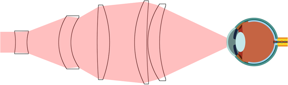
1.IntroductionThe cornea is the front optical element of the human eye and plays a critical role in producing images on the retina. However, the exposed cornea is covered by the tear film, a thin layer of fluid that is 4 to 10 microns thick.1,2 This air–tear film interface contains the largest change in refractive index in the eye, contributing of the eye’s total refractive power. Irregularities in the tear film can result in decreased visual performance,3 physical discomfort,2 and uncomfortable contact lens wear.4 The tear film is also a dynamic surface that rapidly evolves after a blink. In a normal eye, a blink initially destabilizes the tear film and the tear film will rapidly smooth itself over the surface of the cornea within a few seconds due to surface tension of the fluid.5 The tear film will begin to thin after 5 s and may begin to breakup after 15 s.6 Breakup in the tear film typically begins with pits or canyons forming on the surface, which continue to grow in size until the recurrence of another blink. A complete study of the precorneal tear film requires an instrument that is capable of measuring surface topography and thickness distribution of a dynamic film. A common method of evaluating the tear film involves an eye care professional applying a fluorescent fluid to the eye to aide in the inspection of the tear film. The method allows for a simple and qualitative assessment of the tear film thickness, but the installation of a foreign substance is invasive and unreliable for proper tear film characterization.7 A more accurate method for determining tear film thickness can be achieved by measuring the reflectance spectrum that results from a thin-film interference effect with the tear film layers.8,9 Confocal microscopy and optical coherence tomography (OCT) are two additional techniques that have been used to measure the tear film thickness and also have the added benefit of measuring the surface height of the tear film.10,11 However, these methods require lengthy imaging times, which are unfavorable for studying tear film dynamics, have lower thickness resolution than thin-film interference techniques, and lower surface height resolution than the interferometric measurement techniques that are discussed subsequently in this paper. Tear film thickness measurements are useful for studying the structure of the tear film9 and thinning rates following blinks.12 The surface of the tear film is determined by both the underlying corneal shape and tear film thickness distribution. The surface topography of the tear film establishes the first refracting surface of the eye and is important for visual optical quality.3,13 Differential interference contrast microscopy is a method for noninvasive assessment of the tear film surface, but is mainly a qualitative method that evaluates surface slope along a single direction.14 Reflection based corneal topographers (e.g., Placido disks) are able to provide a quantitative measure of the surface topography of the tear film, but lack spatial and height resolution.15,16 Projection based corneal topographers (e.g., Moiré-deflectometry) have better spatial and height resolution than reflection based systems, but are invasive measurements that require the addition of a fluorescing fluid or diffusing agent to the tear film.17,18 Slit scanning systems can measure surface topography and provide additional thickness information within the eye, but also suffer from the same issues as confocal microscopy and OCT techniques.19 Interferometry provides the potential for high-resolution, noninvasive characterization of the tear film surface. The University of Wrocław has conducted a number of studies using interferometry to characterize the in vivo tear film. An initial attempt using a Twyman-Green interferometer to directly measure the surface of the tear film was overly sensitive to eye motion and difficult to align.20 Measurements were captured by a framegrabber at 25 frames per second over a 4.5 mm diameter area on the eye. Surface topography was calculated through fringe tracing and ordering. Fringe densities were generally too high to evaluate, so analysis was limited to covering a 2 mm diameter area on the tear film. However, topography could not be determined with complete certainty; fringe tracing results in lower spatial resolution, reduced height accuracy, and ambiguity in the sign of the topography. This system appears to have been discontinued in favor of lateral shearing interferometry. The advantage of a lateral shearing interferometer is a decreased sensitivity to eye motion, which enabled an increase in measurement area to a 5 mm diameter area on the eye.21–23 Using sufficiently large shear results in a spatial carrier frequency in the recorded interferograms. Phase can be directly recovered using Takeda’s method24 allowing for quantitative reconstruction of the surface topography, unlike the previous Twyman-Green interferometer. However, using shearing to reduce sensitivity to eye motion will decrease both spatial and height resolution. Furthermore, it has been shown that the application of lateral shearing interferometer to in vivo tear film measurements suffers from significant measurement noise due to eye motion.25 The tear film interferometer (TFI) for in vivo measurement of the tear film is an instantaneous phase-shifting Twyman-Green interferometer that has overcome the limitations of its predecessors, increasing the spatial and height resolution of tear film measurements. The TFI system was developed in two phases. The first phase involved the development of an in vitro interferometer system to characterize the dynamic fluid surfaces on contact lenses.26,27 Successful demonstration of the in vitro system led to the development of the TFI, including a detailed study on laser safety.28,29 Since the publications on the initial design, the TFI has been built and approved for testing on human subjects. Feedback from initial human subjects testing has led to numerous improvements in the design. These improvements have resulted in faster alignment times, longer data capture, and improved data quality. 2.Tear Film InterferometerThe TFI is a polarized Twyman-Green interferometer designed to instantaneously measure the wavefront reflected off of the anterior surface of the tear film. The TFI design has been thoroughly described by Primeau and Greivenkamp.28 A schematic of the TFI system is shown in Fig. 1, and a photograph of the completed system is shown in Fig. 2. The laser source is a near-infrared solid-state laser () and is modulated by an acousto-optical modulator (AOM) that is synchronized to the camera’s electronic shutter (refer to Sec. 2.2). A continuously variable neutral density (CVND) filter is used to adjust the laser power level to an eye safe level at the output of the interferometer. Following the laser shutter, a power meter continuously monitors the laser source to ensure eye safe laser levels are maintained at all times. The coherence length of the laser is , requiring optical path matching of the reference and test arms to maximize fringe visibility at the detector. The test path contains a custom-built lens assembly (Photon Gear, Inc., Ontario, New York) to generate a wavefront designed to match the surface shape of the human cornea (Fig. 3). The average corneal shape is best approximated by an asphere having a base radius of 7.8 mm and a conic constant.30 The lens operates at f/1.3, covering a 6 mm diameter on the average human eye. A Stokes lens, or a pair of crossed cylinders, can be placed in the test arm to compensate corneal astigmatism. These are typically left out to minimize stray reflections resulting from one of the four surfaces, but may be necessary for subjects with larger amounts of corneal astigmatism. The reflected wavefront from the tear film surface is interfered with the reference wavefront and detected by a 1 MP Pixelated Camera Kit (4D Technology Corporation, Tucson, Arizona). The camera uses a pixelated phase-mask aligned to the detector array that acquires four phase-shifted interferograms in a single camera frame.31 Phase can be recovered from an individual frame by conventional N-bucket algorithms or spatial convolution methods.31,32 A test subject will sit in front of the TFI and place their head in an ophthalmic headrest (refer to Sec. 2.1.1). The headrest consists of a chin cup, horizontal crossbar with a nose pad to lean their forehead against, and a pair of guiding rods to support the head at the temples. A view looking into the TFI showing the headrest is shown in Fig. 4. The TFI is mounted on top of a pair of linear translation stages that provide fine alignment of the device to the subject. A vertical stage is placed under the headrest for a third degree of fine alignment of the test subject to the interferometer. Eye motion is minimized by using an external fixation with the subject’s dominant eye (green path, Fig. 1) while the other eye is tested. An illuminated target is placed at the focus of a 250 mm focal length lens to present a distant image to the subject. Once the subject fixates on the target, the TFI is aligned to the nondominant eye and measurements are made. Fig. 4View looking into TFI showing the headrest. Configuration shown will test on subject’s left eye with the fixation set for the right eye.  2.1.StabilityOne of the more difficult aspects of measuring the in vivo tear film surface is that it is not a stationary surface that can be firmly mounted and aligned as is typical in most interferometry applications. In addition to the dynamic nature of the tear film, a normal healthy eye will have random, involuntarily motions.33,34 Head motion is another significant source of random motion that will introduce additional motion.35 The dynamic range for the TFI system using the 1 MP pixelated camera, as tested by the manufacturer and verified on the TFI, is waves/radius31 (corresponding to a 22.2 mrad slope error measured at the tear film surface). For a typical measurement, the predicted wavefront slope introduced by eye motion, head motion, and varying ocular geometry is 105 waves/radius28 (13.7 mrad slope error). It should be noted that it was assumed that all motion was centered about a mean position to which the TFI could be aligned. Additionally, it does not include surface slope errors from the tear film surface itself. The initial estimate was that at least 70% of the captured data should be useable, where a useable frame of data is one that was successfully unwrapped (refer to Sec. 3) and contains data dropouts. However, the first tests with the TFI yielded extreme difficulty in aligning to the test subject. Once aligned, only a few seconds of data could be collected, with of the data being useable. The observed motion exceeded all previous predictions and severely limited the functionality of the TFI. The excessive motion that was present during measurements was attributed to two sources: subject stability in the headrest and their inability to maintain sufficient fixation. Although both of these motions were accounted for in the initial design, the sensitivity of the design to these motions was underestimated. This required an iterative approach to redesigning both the headrest and fixation assemblies, which are discussed in the following sections. After the redesign was implemented, a trained operator could align the TFI to a subject in less than a half minute, whereas previously the operator could struggle for minutes. An additional improvement was the quantity of valid data from a given collection increased from to . Furthermore, there has been no determinable limit to the duration of a data collection, with acquisition times up to 120 s having been repeatedly demonstrated. Duration is limited by subject fatigue rather than the previous limitation where subject motion exceeded the dynamic range of the TFI. 2.1.1.Head stabilizationThe TFI head stabilization fixture (Fig. 4) is a modified reproduction of a commercial head positioning system from Arrington Research (Scottsdale, Arizona). The commercial system was found to have insufficient stability for this application, so the modifications involve strengthening critical components. The current fixture now consists of a pair of vertically mounted 1 ft. tall, 1.5 in. diameter, dampened steel posts, securely mounted to a base plate. The chin cup and forehead rest were rapid prototyped out of glass-filled nylon and tripled in thickness from the original parts. An aluminum rod is also used to connect the two posts along the top to further constrain lateral motion. The pair of 0.5 in. black guiding rods from the original device has been reused; they are not critical to the overall stability of the fixture, but are still necessary to maintain subject stability. These guiding rods do not physically constrain the subject’s head, but act as a physiological reminder for the subject to hold their head still. At any point during the test, the subject can back out of the headrest with little effort. Finally, the layout was adjusted to place the subject’s head to rest as close to the base of the fixture as possible, reducing the significant moment arm that previously existed. 2.1.2.FixationFixation of the eye is accomplished by directing the subject to lock their visual gaze on a stationary target. Despite the subject’s attempt to maintain fixation, their eyes will naturally make small, involuntary motions. These eye motions are composed of three movement types: saccades (quick, large flicks of the eye), drifts (slow, cyclic motions), and physiological nystagmus or tremors (small, random, high-frequency motions).36 Previous studies have shown that color, luminance, contrast, or image quality of the fixation target have no effect on fixation except in the case where any of these factors render the target barely visible.37,38 However, it was found that differences in fixation target sizes resulted in changes in saccades and drift.38,39 Some studies have concluded that the optimal fixation target shape to minimize random eye movement is a set of cross-hairs surrounded by a circular target with a dot in the center.40 External distractions, such as motion in the peripheral vision or auditory stimuli, were also found to increase the amount of microsaccades.41,42 There is an important distinction between the TFI fixation and the systems described in the literature: the TFI uses monocular off-eye fixation, whereas the systems described in the literature used monocular on-eye fixation. In the original implementation, the fixation target was an image of the Old Main building on the University of Arizona campus [Fig. 5(a)]. In an attempt to improve fixation stability, the experiments of Boyce37 and Steinman et al.38 were replicated to verify the optimal choice of fixation targets. The experiment was modified to account for the off-eye fixation used on the TFI, such that eye tracking system would monitor the eye under test while the subject performed monocular fixation with the opposite eye. A commercial eye tracker (Arrington Research, Scottsdale, Arizona) is attached to the side of the converger optics and images the eye at a 45-deg angle. Subjects were placed in front of the TFI in a normal test configuration, with the exception that the TFI laser was disabled. Subjects were then instructed to fixate on a series of different targets (Fig. 5) for up to 2 min. Additionally, subjects were tested with different permutations of illumination schemes: red, green, blue, and white illumination; low or high illumination; and constant or modulated illumination. A total of six subjects were tested with the eye tracking system. The results were in good agreement with the previous tests of Boyce and Steinman; the largest contributor to eye motion was the target shape. Target performance is ordered in Fig. 5 with the worst starting on the left (image of the Old Main building) to the best performing on the right (cross-hairs with circle). The improvement gained by switching from the image of the building to the cross-hairs was a decrease in random eye motion by 50%. The distribution shown in Fig. 6 is from a single test subject but is representative of every subject tested. Although more difficult to quantify due to the limited data, it appears as though saccades were also reduced 50% by choice of the cross-hair target. Fig. 6Eye motion during target fixation. Histogram shows radial deviation from mean position. (a) Fixation on image of building and (b) fixation on cross-hairs with circle. Gaze direction was not calibrated for absolute positions; therefore, the axes are normalized from 0 to 1.  Although Steinman38 reports no variation for illumination color, he did not test the color blue. Based on our test results, we saw an increase in eye motion for targets that were illuminated with a solid blue light. Otherwise, all other color schemes were in agreement with Steinman, producing negligible variation in eye motion. When given a choice, most subjects chose a constant green illumination. Therefore, the implemented illumination system uses a fixed, constant green illumination scheme with the cross-hair target. Finally, baffling was added to the TFI to minimize peripheral distractions. The front panel of the TFI enclosure was originally a specular black plastic panel that subjects could see directly in front of them when testing. This panel was replaced by a diffuse black panel. Instrumentation displays, such as the power meter, were easily visible by the subject when sitting in front of the instrumentation. Black diffuse panels were placed on both sides of the subject. These structures can be seen in Fig. 4. Although no empirical data have been collected on the use of baffles, it is expected to provide a benefit based on previous studies.41,42 2.2.Interferometer Source ModulationSource modulation was not implemented in the original design of the interferometer. It was thought that the 785 nm wavelength laser source was sufficiently below the human visual response that modulation would be unnecessary. However, every test subject has reported being able to see the 785 nm source, which is focused to be concentric with the cornea. Subjects report that the source appears as a large, faint, dark red spot that fills their vision and is filled with smaller blobs that were either static or moving across their field of vision. It is speculated that the static blobs were a combination of dust particles within the interferometer and floaters in the subject’s eye. Moving structures were reported to move downward, which would be consistent with the observed tear film dynamics. Upon blinking, the tear film would be pulled upward by surface tension and the upper lid. The perceived downward motion of the structures is a result of an inverted image due to the source coming to focus inside the eye. Because the laser source subtends 45 deg of the subject’s field, resulting in significant peripheral distraction, visual perception of the source must be minimized to guarantee stable fixation during testing. The first attempt at correction was to reduce the laser power and increase camera gain. However, even at the lowest practical levels, or at the surface of the cornea, the source was still perceptible to most subjects. Therefore, an obvious next step was to modulate the laser source. The laser was modulated by placing an AOM directly after the laser source with the modulation synchronized to the camera’s electronic shutter. The nominal camera frame rate operates at 33 ms with camera integration times limited to , resulting in duty cycle of laser source illumination. Once the laser source was modulated, subjects reported no longer being able to see the laser source. Modulating the laser source provides an added benefit: a reduction in detector blooming and subsequently an increase in fringe modulation. The detector in the 4D pixelated camera (Truesense Imaging KAI-1010) specifies blooming suppression to be , which is sufficient for nominal operation. However, the large fringe densities that are measured at the detector, which are a result of eye motion, ocular variation, misalignment, and tear film dynamics, are significantly reduced in modulation by detector sampling.43 By modulating the source and reducing blooming, fringe modulation can be improved by as much as 10%. 3.Data AnalysisOnce a sequence of data is captured, a series of operations take place to recover the surface topography of the tear film. A brief summary of the operations required to recover the surface is shown in Fig. 7. A more in-depth discussion of the process can be found in Sec. 14.15 of Ref. 44. However, two operations require special attention for the operation of the TFI: phase unwrapping and surface correction. 3.1.Phase UnwrappingThe use of the pixelated phase mask camera allows four simultaneous frames of phase-shifted data to be captured. Standard phase recovery algorithms can be applied to the instantaneous frame to recover the phase.45 A single frame extracted from a measurement made on the TFI is shown in Fig. 8(a) along with the recovered phase [Fig. 8(b)]. Because the recorded interferograms are a cyclical function of the measured phase, the recovered phase will be a modulo of the true phase. The process of removing discontinuities and recovering the surface is known as phase unwrapping and is a widely researched topic.46 Conventional interferometric testing typically results in data with high signal-to-noise ratios and minimal defects in the image. This reduces the burden on the phase unwrapping process, which tend to be sensitive to noise and defects in the phase surface. However, the tear film surface is unlike most optical surfaces. First, the structure of the tear film contains a large amount of mid- to high-spatial frequency content. This becomes an issue when structures exceed the dynamic range of the instrument, generally where tear film breakup occurs, or when mucus globules or other particles appear in the tear film surface. Eye disease, such as dry eye syndrome, may increase the prevalence of mid- to high-spatial frequency structures. These structures have to be avoided or minimally processed during the phase unwrapping routine. Second, since the TFI data are processed on a frame-by-frame basis, eye motion will induce a significant amount of tilt and defocus, further increasing fringe density in a given frame of data. Finally, ocular variation will contribute additional low-order surface features, typically astigmatism and spherical aberration. The interaction of all these effects will generate dense fringe patterns on the detector that are reduced in modulation by detector sampling. Reduced modulation will result in reduced signal, increasing the difficulty of a successful phase unwrapping. An example breakdown during phase unwrapping is shown in Fig. 9(a). The discontinuities result from the phase unwrapping algorithm’s failure to properly resolve discontinuities. Path following algorithms, where pixels are processed from a neighborhood queue, tend to propagate these errors across the rest of the image. A successful phase unwrapping of the same data is shown in Fig. 9(b). Fig. 9(a) Example of surface with phase unwrapping errors and (b) same surface processed with a more robust phase unwrapping algorithm. Note: the surface on the left was processed with a different application than on the right, resulting in different color maps.  Two algorithms have been successfully implemented in phase unwrapping TFI data. The first algorithm is more generally known as a quality-guided phase unwrapping algorithm.47,48 Quality-guided unwrapping routines utilize a quality metric to determine the path of unwrapping in the recovered two-dimensional wrapped phase image. When generating the queue of neighboring pixels to be unwrapped, the ordering is determined by the quality map and higher-quality pixels are given priority. Phase-shifting interferometry allows for the recovery of a modulation map, which has been shown to be a useful quality metric.48 However, the typical measured fringe densities in a TFI image result in low modulation across large areas, negating the advantage of a modulation map. It was found that the modulation quality map could be supplemented with a local slope variance map, similar to previous methods.47 The initial phase slope along the - direction is defined as the forward difference of the measured phase at a pixel location : The unwrapped phase will contain phase discontinuities, which can be removed from the initial slope to determine a proper slope estimate : A neighborhood mean of phase slopes , where , can be determined: The directional phase derivative variance is then given by the expression The same math can be applied to solve for the directional phase derivative variance along the direction [], and the total phase derivative variance can be given by Predictions of slope variance can be improved by weighting the average using the modulation quality map. The quality metric for slope variance can then be derived as an inverse of local slope variance, for example. An example of a quality guided algorithm using both modulation and slope variance quality metrics to unwrap the phase is shown on the right in Fig. 9. Quality guided phase unwrapping methods using modulation and slope variance as quality metrics have been successful at handling most of the data collected with the TFI. The remaining set of data that cannot be processed with the quality guided method can usually be ignored. This type of data usually occurs around a saccade or when the subject’s fixation drifts momentarily, and will only exist for one or two frames. However, there are cases where data sets may have extreme surface features that need to be recovered. In these instances, a more robust algorithm is used to unwrap the data sets. An example of a more extreme set of data is shown in Fig. 10. The surface data on the left was unwrapped using the quality guided method as described previously and could only handle a small region before breaking down in the exterior regions. Fig. 10An example extreme data set: (a) unwrapped using quality-guided method and (b) unwrapped using a preconditioned conjugate gradient method. 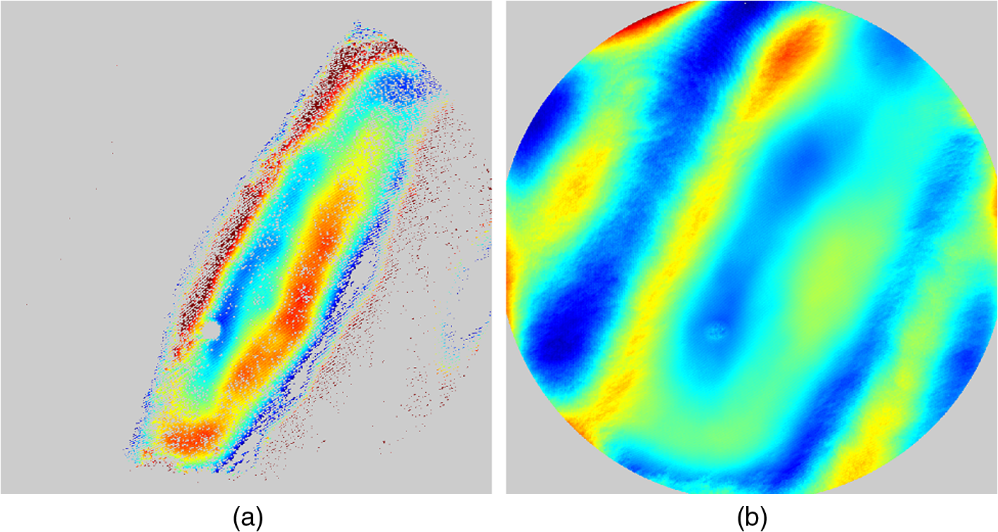 The second, more robust, phase unwrapping algorithm uses a preconditioned conjugate gradient (PCG) method to minimize the difference between the gradients of the wrapped and unwrapped phases.46,49 The weighted least-squares solution to this minimization problem reduces to Poisson’s equation, which can be solved by a number of means.50 The least-squares solution has a closed-form solution that can be solved using fast Fourier transforms, but will only be useful as an initial guess for the final surface solution. The same quality map from the quality guided routine can be applied as a weighting. The preconditioned conjugate gradient method is then used to iteratively solve for a surface solution. Figure 10 shows the same surface being unwrapped with the quality guided method [Fig. 10(a)] and the PCG method [Fig. 10(b)]. This method has two main advantages over the quality guided method. The first is that it is a global phase unwrapping process; noise defects that appear in the middle of an image will not be propagated throughout the image as they would be in a path-following method. The second is that it accepts a quality map, which ensures convergence to a proper surface solution. However, the major disadvantage of the PCG method is that it requires approximately four times the amount of processing time over the quality guided method. Therefore, the PCG method is only used sparingly. 3.2.Surface CorrectionWhen interferometrically testing optical components, it may be common for residual wavefront errors to show up in the measured wavefront due to a misalignment of the test surface with respect to the interferometer. For example, testing a decentered spherical part will show up as a tilt in the measured wavefront. Knowing that tilt is an artifact of an alignment error and not actually representative of the test surface, it is considered acceptable to subtract the tilt in postprocessing of the wavefront. As a result, a first approximation to correct the TFI data for eye motions between frames would be to simply subtract the average tilt from each frame. Since the goal of the TFI is to measure the mid- and higher-spatial frequency variations of the tear film, the measured power can also be subtracted. However, postprocessing of tear film surface measurements will become more complicated by the extreme ranges of data collected. When removing measurement terms, such as tilt or power due to alignment, it is assumed that the wavefront was near null and the measured fringe densities were minimal. Larger displacements of the test surface and greater surface deviations will increase fringe densities and result in a non-null condition. When the null condition is violated, the wavefront measured at the detector is no longer representative of the test surface.51 In other words, subtraction of tilt and power is no longer sufficient to recover the actual test surface. The error that is accumulated on the measured wavefront is a result of the test wavefront passing through different portions of the interferometer optics than what the null wavefront would have propagated through. This systematic error is commonly referred to as retrace error. In ray tracing terms, it is the difference in path that a non-null test ray takes through the interferometer optics than that of a null ray.52 The dominant component of retrace error is referred to in literature as a shearing or phase error.53,54 When considering the fact that the interferometer is imaging the test object’s surface onto the detector, the systematic errors introduced by the interferometer can be described in terms of imaging aberrations. Because the source is spatially filtered, the phase across any detector pixel can be accurately represented by a single ray that maps to the test surface. Therefore, the phase error is equivalently the wavefront error for the given field height and pupil coordinate . Because this is a single ray that results from a reflection off of the test surface, the pupil location can be completely described by the surface departure. where represents the surface sag in radial coordinates , is the gradient, and represents the nominal marginal ray slope.As an example, we will consider the effect of eye motion in the TFI. The largest imaging aberration present in the TFI is distortion and the wavefront aberration can be defined by standard aberration theory. where is the distortion coefficient. The largest component of eye motion is in the lateral direction, which will introduce tilt in the wavefront. Lateral motion of the test surface will shift all pupil intercepts equally in the same direction by twice the amount of eye decenter :The phase error is where the constant is defined asThe phase error will show up as coma in the surface that is scaled by the system parameters and surface decenter. For the TFI system, . In other words, every of decenter of the eye will generate an additional wave of coma that will show up in the measured surface. With the expected range of eye motion of , tear film surface data will contain coma that can vary over a range of waves. Based on the aforemetioned result, an initial thought would be to remove tilt and an amount of coma that is scaled by the magnitude of tilt present. However, this would be incorrect. The previous example only considered distortion in the imaging system and lateral displacement of the eye. A full analysis including all of the TFI image system aberrations, eye motions, and ocular variations would yield a number of cross-terms that would not allow for a straightforward correction. Furthermore, it would be difficult, if not impossible, to separate surface features from introduced phase error. When the full analysis was applied to the TFI to determine the parameters that are most sensitive to eye motion, it was found that the first eight Zernike polynomial terms [Tilt (x2), Power, Astigmatism (x2), Coma (x2), and Spherical) are sufficient. In other words, to view the dynamic surface topography of the tear film, which does not contain random surface fluctuations that are a result of eye motion and retrace errors, the first eight Zernike polynomial terms should be removed. Trefoil and secondary astigmatism, the next four Zernike terms, are weakly affected by retrace errors and do not necessarily have to be removed. However, additional Zernike terms may be removed to enhance the display of higher spatial frequency structure in the tear film. The number of Zernike terms removed would have to be determined by the individual subject’s unique corneal topography. Data collected from most of the subjects tested to date have topographies that necessitated the removal of the first 12 Zernike terms, with the largest requiring the first 19 Zernike terms to be removed. By removing these terms, the measured corneal surface is effectively projected onto a plane that allows for high-resolution inspection of the dynamic tear film structure over the desired range of spatial frequencies. 4.ResultsTo date, seven human subjects have been examined using the TFI. Testing on human subjects has been approved by the University of Arizona institutional review board and adheres to the tenants of the Declaration of Helsinki. Informed consent is obtained from a subject prior to testing. Testing was performed on healthy adults, aged 18 to 60 years. Subjects were not allowed to participate if they had any known eye disease or have undergone refractive surgery. Subjects outside of this age range or with an eye disease may introduce potential complications that inhibit the TFI system’s ability to collect data. A trained operator can align the TFI to a subject in under a minute. Acquisition times up to 120 s have been repeatedly demonstrated with no appreciable change in data quality. Subjects will sit an average of 5 min in the TFI before requiring a small break; the TFI will have to be realigned upon resumption of testing. Test protocol limits the total time with a subject to 60 min. However, subject fatigue becomes noticeable after 20 to 30 min at which point the test is ended. In a typical data set, of the frames captured will be useable. The other 10% of data is lost due to transient events, such as large saccades or drifts that move the cornea out of interferometer capture range, saccadic motion that is faster than the camera exposure time, blinking (i.e., eyelid and eyelashes obstruct the cornea), loss of fixation that occurs around a blink, and rapid axial motion of the eye during a blink.55 The reconstructed surface topography has an average lateral resolution of , surface height resolution better than or 25 nm, and 35 ms temporal resolution of dynamic surface features. A small subset of data that has been collected from the TFI is shown in Figs. 11Fig. 12Fig. 13Fig. 14–15 and includes links to the video sources. The interferogram shown in Fig. 11 (Video 1) is dominated by tilt and defocus as a result of eye and head motion, where axial motion of the subject results in defocus and lateral motion results in tilt. Figure 12 (Video 2) shows the reconstructed surfaces from the series of interferograms in Fig. 11. The peak-to-valley (PV) scale for Fig. 12 is , with red representing high or away from the surface of the eye. The surface data have had the first 12 Zernike polynomials removed to enhance the display of mid- to high-spatial frequency information.56 The removal of the first 12 Zernike terms was sufficient for all of the examples given in this paper to minimize the effects of subject motion (first eight terms) and topography that would dominate the dynamic range of the display (next four terms). The topography at the start of (Video 2) Fig. 12 is indicative of a partial blink, which results in the large horizontal valley formation at the lower third of the display. A second partial blink occurs approximately 2 s into the video and results in a secondary horizontal valley at the upper third of the display. The topography of the partial blink bears strong resemblance to tear film thickness measurements that have been reported in the literature.13 Fig. 11Interferogram data. Partial blink occurs at 2 s. Area shown is . Note: videos are heavily compressed for website. Video 1 (MPEG, 3.9 MB) [URI: http://dx.doi.org/10.1117/1.JBO.20.5.055007.1].  Fig. 12Reconstructed surface from interferograms in Fig. 11. First 12 Zernike terms have been removed. PV scale is , red is high (away from eye). Video 2 (MPEG, 4.1 MB) [URI: http://dx.doi.org/10.1117/1.JBO.20.5.055007.2].  Fig. 13Evolution of tear film over 45 s: (a) 1 s after blink and (b) 45 s after blink. Upper eyelid and an eyelash can be seen at the top of the data. Data scale is PV, red is high; 12 Zernike terms removed. Video starts directly after a blink and ends at the occurrence of the next blink. Video 3 (MPEG, 4.9 MB) [URI: http://dx.doi.org/10.1117/1.JBO.20.5.055007.3].  Fig. 14Subject exhibiting high spatial frequency structures after blink. Blinks occur at 0 and 6 s. Data scale is PV, red is high; 12 Zernike terms removed Video 4 (MPEG, 3.9 MB) [URI: http://dx.doi.org/10.1117/1.JBO.20.5.055007.4].  Fig. 15Subject exhibiting low spatial frequency structures after blink. Blinks occur at 3, 4, and 16 s. Data scale is PV, red is high; 12 Zernike terms removed Video 5 (MPEG, 4.4 MB) [URI: http://dx.doi.org/10.1117/1.JBO.20.5.055007.5]. 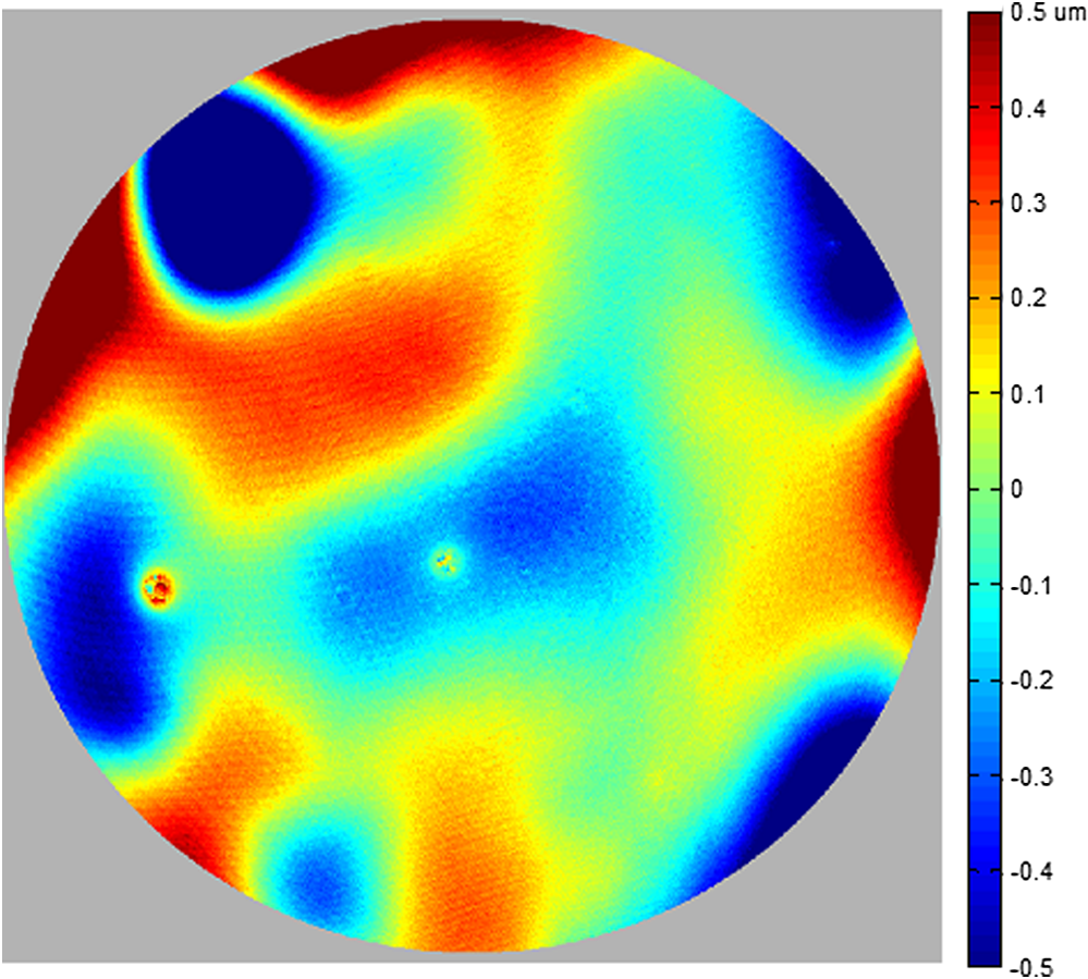 An example of a stable tear film is shown in Fig. 13 (Video 3), where a subject was able to maintain gaze for 45 s before blinking. The tear film is stabilized within a second after a blink, which is where the still on the left is taken from. The still on the right shows the tear film after 45 s without a blink occurring. The tear film has become more irregular and contains larger surface height features as tear film breakup and evaporation occurs due to being exposed to air. Figure 14 (Video 4) is taken from a subject that exhibits high is taken from a subject that exhibits high spatial frequency structures in the tear film, which form quickly after blinking. The magnitude of these structures is greater than previous examples, so the dynamic range of the display was increased to . A similar example of a subject exhibiting large dynamic structures occurring after a blink is shown in Fig. 15 (Video 5). However, these structures are lower in spatial frequency compared to Fig. 14 and are not consistent after the subject blinks. Additional features of the tear film dynamics can also be observed in the video data, including postblink dynamics, evaporation, breakup, and the propagation of foreign objects in the tear film. 5.ConclusionsThe TFI has been demonstrated as a viable and practical technology for the noninvasive characterization of the dynamic topography of the in vivo corneal tear film. Several human subjects have been examined using this system, with a demonstrated surface height resolution of 25 nm and spatial resolution of . Acquisition times of up to 120 s have been obtained. The combination of height resolution, spatial resolution, and measurement area has been improved over existing in vivo technologies. Preliminary data that have been shown to the medical community have generated interest. However, data collection has only been performed on a small subset of people to verify its capabilities. Future testing is expected to be performed within a clinical setting where the dynamic topography can be correlated to physiological conditions. ReferencesS. Mishima,
“Some physiological aspects of the precorneal tear film,”
Arch. Ophthalmol., 73
(2), 233
–241
(1965). http://dx.doi.org/10.1001/archopht.1965.00970030235017 AROPAW 0003-9950 Google Scholar
F. J. Holly,
“Tear film physiology,”
Am. J. Optom. Physiol. Opt., 57
(4), 252
–257
(1980). http://dx.doi.org/10.1097/00006324-198004000-00008 AOPOCF 0093-7002 Google Scholar
H. T. Kasprzak and T. Licznerski,
“Influence of the characteristics of tear film break-up on the point spread function of an eye model,”
Proc. SPIE, 3820 390
–396
(1999). http://dx.doi.org/10.1117/12.353091 PSISDG 0277-786X Google Scholar
J. P. Guillon,
“Tear film structure and contact lenses,”
The Preocular Tear Film in Health, Disease and Contact Lens Wear, 914
–939 Dry Eye Institute, Lubbock, Texas
(1986). Google Scholar
D. Benedetto, T. E. Clinch and P. R. Laibson,
“In vivo observation of tear dynamics using fluorophotometry,”
Arch. Ophthalmol., 102
(3), 410
–412
(1984). http://dx.doi.org/10.1001/archopht.1984.01040030328030 AROPAW 0003-9950 Google Scholar
J. Németh et al.,
“High-speed videotopographic measurement of tear film build-up time,”
Invest. Ophthalmol. Vis. Sci., 43
(6), 1783
–1790
(2002). IOVSDA 0146-0404 Google Scholar
S. Patel et al.,
“Effects of fluorescein on tear breakup time and on tear thinning time,”
Am. J. Optom. Physiol. Opt., 62
(3), 188
–190
(1985). http://dx.doi.org/10.1097/00006324-198503000-00006 AOPOCF 0093-7002 Google Scholar
N. Fogt, P. E. King-Smith and G. Tuell,
“Interferometric measurement of tear film thickness by use of spectral oscillations,”
JOSA A, 15
(1), 268
–275
(1998). http://dx.doi.org/10.1364/JOSAA.15.000268 JOAOD6 1084-7529 Google Scholar
P. E. King-Smith et al.,
“Interferometric imaging of the full thickness of the precorneal tear film,”
JOSA A, 23
(9), 2097
–2104
(2006). http://dx.doi.org/10.1364/JOSAA.23.002097 JOAOD6 1084-7529 Google Scholar
J. I. Prydal and F. W. Campbell,
“Study of precorneal tear film thickness and structure by interferometry and confocal microscopy,”
Invest. Ophthalmol. Vis. Sci., 33
(6), 1996
–2005
(1992). IOVSDA 0146-0404 Google Scholar
W. Drexler et al.,
“Ultrahigh-resolution ophthalmic optical coherence tomography,”
Nat. Med., 7
(4), 10
–15
(2001). http://dx.doi.org/10.1038/86589 1078-8956 Google Scholar
J. J. Nichols, G. L. Mitchell and P. E. King-Smith,
“Thinning rate of the precorneal and prelens tear films,”
Invest. Ophthalmol. Vis. Sci., 46
(7), 2353
–2361
(2005). http://dx.doi.org/10.1167/iovs.05-0094 IOVSDA 0146-0404 Google Scholar
R. J. Braun et al.,
“Dynamics and function of the tear film in relation to the blink cycle,”
Prog. Retin. Eye Res., 45 132
–164
(2015). http://dx.doi.org/10.1016/j.preteyeres.2014.11.001 PRTRES 1350-9462 Google Scholar
H. Hamano et al.,
“Clinical applications of bio differential interference microscope,”
Eye Contact Lens, 6
(3), 229
–235
(1980). 1542-2321 Google Scholar
D. Priest and R. Munger,
“Comparative study of the elevation topography of complex shapes,”
J. Cataract Refract. Surg., 24
(6), 741
–750
(1998). http://dx.doi.org/10.1016/S0886-3350(98)80125-9 JCSUEV 0886-3350 Google Scholar
C. J. Roberts,
“Comparison of the EyeSys corneal analysis system and the TMS topographic modeling system using a bicurve test surface,”
Proc. SPIE, 2126 168
–173
(1994). http://dx.doi.org/10.1117/12.178582 PSISDG 0277-786X Google Scholar
F. H. M. Jongsma et al.,
“Development of a wide field height eye topographer: validation on models of the anterior eye surface,”
Optom. Vis. Sci., 75
(1), 69
–77
(1998). http://dx.doi.org/10.1097/00006324-199801000-00027 OVSCET 1040-5488 Google Scholar
W.-Y. Chang et al.,
“Heterodyne Moiré interferometry for measuring corneal surface profile,”
Opt. Lasers Eng., 54 232
–235
(2014). http://dx.doi.org/10.1016/j.optlaseng.2013.07.013 OLENDN 0143-8166 Google Scholar
G. Cairns et al.,
“Accuracy of Orbscan II slit-scanning elevation topography,”
J. Cataract Refract. Surg., 28
(12), 2181
–2187
(2002). http://dx.doi.org/10.1016/S0886-3350(02)01504-3 JCSUEV 0886-3350 Google Scholar
T. J. Licznerski, H. T. Kasprzak and W. Kowalik,
“Application of Twyman–Green interferometer for evaluation of in vivo breakup characteristic of the human tear film,”
J. Biomed. Opt., 4
(1), 176
–182
(1999). http://dx.doi.org/10.1117/1.429904 JBOPFO 1083-3668 Google Scholar
H. T. Kasprzak, W. Kowalik and J. Jaroński,
“Interferometric measurements of fine corneal topography,”
Proc. SPIE, 2329 32
–39
(1995). http://dx.doi.org/10.1117/12.200907 PSISDG 0277-786X Google Scholar
T. J. Licznerski, H. T. Kasprzak and W. Kowalik,
“Two interference techniques for in-vivo assessment of the tear film stability on a cornea and contact lens,”
Proc. SPIE, 3320 183
–186
(1998). http://dx.doi.org/10.1117/12.301335 PSISDG 0277-786X Google Scholar
T. J. Licznerski and H. T. Kasprzak,
“Reconstruction of the corneal topography from lateral-shearing interferograms,”
Proc. SPIE, 3820 115
–119
(1999). http://dx.doi.org/10.1117/12.353049 PSISDG 0277-786X Google Scholar
M. Takeda, H. Ina and S. Kobayashi,
“Fourier-transform method of fringe-pattern analysis for computer-based topography and interferometry,”
JOSA, 72
(1), 156
–160
(1982). http://dx.doi.org/10.1364/JOSA.72.000156 JSDKD3 Google Scholar
A. Dubra, C. Paterson and C. Dainty,
“Study of the tear topography dynamics using a lateral shearing interferometer,”
Opt. Express, 12
(25), 6278
–6288
(2004). http://dx.doi.org/10.1364/OPEX.12.006278 OPEXFF 1094-4087 Google Scholar
B. C. Primeau and J. E. Greivenkamp,
“Interferometer and analysis methods for the in vitro characterization of dynamic fluid layers on contact lenses,”
Opt. Eng., 51
(6), 063601
(2012). http://dx.doi.org/10.1117/1.OE.51.6.063601 OPEGAR 0091-3286 Google Scholar
B. C. Primeau, J. E. Greivenkamp and J. J. Sullivan,
“In vitro interferometric characterization of dynamic fluid layers on contact lenses,”
Proc. SPIE, 8133 81330J
(2011). http://dx.doi.org/10.1117/12.892830 PSISDG 0277-786X Google Scholar
B. C. Primeau and J. E. Greivenkamp,
“Interferometer for measuring the dynamic surface topography of a human tear film,”
Proc. SPIE, 8215 821504
(2012). http://dx.doi.org/10.1117/12.907083 PSISDG 0277-786X Google Scholar
B. C. Primeau, G. L. Goldstein and J. E. Greivenkamp,
“Laser exposure analysis for a near-infrared ocular interferometer,”
Opt. Eng., 51
(6), 064301
(2012). http://dx.doi.org/10.1117/1.OE.51.6.064301 OPEGAR 0091-3286 Google Scholar
P. M. Kiely, G. Smith and L. G. Carney,
“The mean shape of the human cornea,”
J. Mod. Opt., 29
(8), 1027
–1040
(1982). http://dx.doi.org/10.1080/713820960 JMOPEW 0950-0340 Google Scholar
J. E. Millerd et al.,
“Pixelated phase-mask dynamic interferometer,”
Proc. SPIE, 5531
(520), 304
–314
(2004). http://dx.doi.org/10.1117/12.560807 PSISDG 0277-786X Google Scholar
. Z. Malacara and M. Servín, Interferogram Analysis for Optical Testing, 2nd ed.CRC Press, Boca Raton, FL
(2010). Google Scholar
H. B. Barlow,
“Eye movements during fixation,”
J. Physiol., 116
(3), 290
–306
(1952). http://dx.doi.org/10.1113/jphysiol.1952.sp004706 JPHYA7 0022-3751 Google Scholar
F. Ratliff and L. A. Riggs,
“Involuntary motions of the eye during monocular fixation,”
J. Exp. Psychol., 40
(6), 687
–701
(1950). http://dx.doi.org/10.1037/h0057754 JEPSAK 0022-1015 Google Scholar
H. T. Kasprzak and D. R. Iskander,
“Ultrasonic measurement of fine head movements in a standard ophthalmic headrest,”
IEEE Trans. Instrum. Meas., 59
(1), 164
–170
(2010). http://dx.doi.org/10.1109/TIM.2009.2022431 IEIMAO 0018-9456 Google Scholar
R. M. Steinman et al.,
“Miniature eye movement,”
Science, 181
(4102), 810
–819
(1973). http://dx.doi.org/10.1126/science.181.4102.810 SCIEAS 0036-8075 Google Scholar
P. R. Boyce,
“The effect of change of target field luminance and colour on fixation eye movements,”
Opt. Acta (Lond)., 14
(3), 213
–217
(1967). http://dx.doi.org/10.1080/713818033 OPACAT 0030-3909 Google Scholar
R. M. Steinman,
“Effect of target size, luminance, and color on monocular fixation,”
JOSA, 55
(9), 1158
–1165
(1965). http://dx.doi.org/10.1364/JOSA.55.001158 JSDKD3 Google Scholar
J. D. Rattle,
“Effect of target size on monocular fixation,”
Opt. Acta (Lond)., 16
(2), 183
–192
(1969). http://dx.doi.org/10.1080/713818162 OPACAT 0030-3909 Google Scholar
L. Thaler et al.,
“What is the best fixation target? The effect of target shape on stability of fixational eye movements,”
Vision Res, 76 31
–42
(2013). http://dx.doi.org/10.1016/j.visres.2012.10.012 VISRAM 0042-6989 Google Scholar
R. Engbert and R. Kliegl,
“Microsaccades uncover the orientation of covert attention,”
Vision Res, 43
(9), 1035
–1045
(2003). http://dx.doi.org/10.1016/S0042-6989(03)00084-1 VISRAM 0042-6989 Google Scholar
M. Rolfs, R. Engbert and R. Kliegl,
“Crossmodal coupling of oculomotor control and spatial attention in vision and audition,”
Exp. Brain Res., 166
(3–4), 427
–439
(2005). http://dx.doi.org/10.1007/s00221-005-2382-y EXBRAP\ 0014-4819 Google Scholar
J. D. Gaskill, Linear Systems, Fourier Transforms, and Optics, Wiley, New York
(1978). Google Scholar
D. Malacara, Optical Shop Testing, 3rd ed.John Wiley & Sons, Hoboken, NJ
(2007). Google Scholar
B. T. Kimbrough,
“Pixelated mask spatial carrier phase shifting interferometry algorithms and associated errors,”
Appl. Opt., 45
(19), 4554
–4562
(2006). http://dx.doi.org/10.1364/AO.45.004554 APOPAI 0003-6935 Google Scholar
D. C. Ghiglia and M. D. Pritt, Two-Dimensional Phase Unwrapping: Theory, Algorithms, and Software, Wiley, New York, NY
(1998). Google Scholar
D. J. Bone,
“Fourier fringe analysis: the two-dimensional phase unwrapping problem,”
Appl. Opt., 30
(25), 3627
–3632
(1991). http://dx.doi.org/10.1364/AO.30.003627 APOPAI 0003-6935 Google Scholar
Y. Xu and C. Ai,
“Simple and effective phase unwrapping technique,”
Proc. SPIE, 253 254
–263
(2003). http://dx.doi.org/10.1117/12.165458 PSISDG 0277-786X Google Scholar
D. C. Ghiglia and L. A. Romero,
“Robust two-dimensional weighted and unweighted phase unwrapping that uses fast transforms and iterative methods,”
JOSA A, 11
(1), 107
–117
(1994). http://dx.doi.org/10.1364/JOSAA.11.000107 JOAOD6 1084-7529 Google Scholar
D. C. Ghiglia and L. A. Romero,
“Minimum Lp-norm two-dimensional phase unwrapping,”
JOSA A, 13
(10), 1999
–2013
(1996). http://dx.doi.org/10.1364/JOSAA.13.001999 JOAOD6 1084-7529 Google Scholar
A. E. Lowman and J. E. Greivenkamp,
“Interferometer errors due to the presence of fringes,”
Appl. Opt., 35
(34), 6826
–6828
(1996). http://dx.doi.org/10.1364/AO.35.006826 APOPAI 0003-6935 Google Scholar
L. A. Selberg,
“Interferometer accuracy and precision,”
Proc. SPIE, 1400 24
–32
(1991). http://dx.doi.org/10.1117/12.26110 PSISDG 0277-786X Google Scholar
C. Huang,
“Propagation errors in precision Fizeau interferometry,”
Appl. Opt., 32
(34), 7016
–7021
(1993). http://dx.doi.org/10.1364/AO.32.007016 APOPAI 0003-6935 Google Scholar
P. E. Murphy, T. G. Brown and D. T. Moore,
“Interference imaging for aspheric surface testing,”
Appl. Opt., 39
(13), 2122
–2129
(2000). http://dx.doi.org/10.1364/AO.39.002122 APOPAI 0003-6935 Google Scholar
M. G. Doane,
“Interaction of eyelids and tears in corneal wetting and the dynamics of the normal human eyeblink,”
Am. J. Ophthalmol., 89
(4), 507
–516
(1980). http://dx.doi.org/10.1016/0002-9394(80)90058-6 AJOPAA 0002-9394 Google Scholar
J. C. Wyant and K. Creath,
“Basic wavefront aberration theory for optical metrology,”
Appl. Opt. Opt. Eng., Xl 1
–53
(1992). AOOEDF 0197-8535 Google Scholar
BiographyJason D. Micali is currently working on his PhD degree in optical sciences from the College of Optical Sciences at the University of Arizona, where he received his MS degree in 2012. His interests include electro-optical systems, interferometry and optical testing, and metrology. John E. Greivenkamp is a professor at the College of Optical Sciences at the University of Arizona. He has served as a member of the SPIE Board of Directors and also as the editor of the SPIE Field Guide Series. He is the author of SPIE Field Guide to Geometrical Optics. Brian C. Primeau received his PhD degree in optical sciences from the University of Arizona in 2011 and is now part of the technical staff at the Massachusetts Institute of Technology Lincoln Laboratory as an optical systems engineer. His interests are in optical system design, metrology, and novel applications of interferometry. |