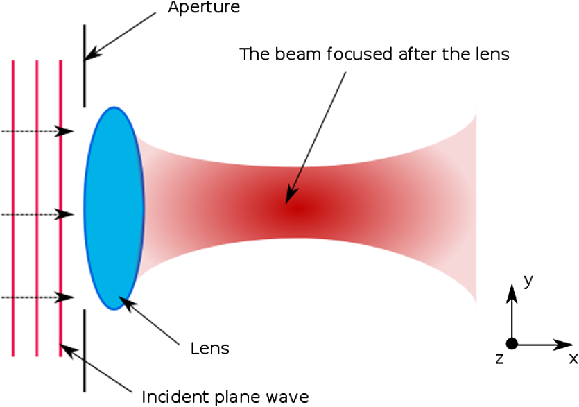
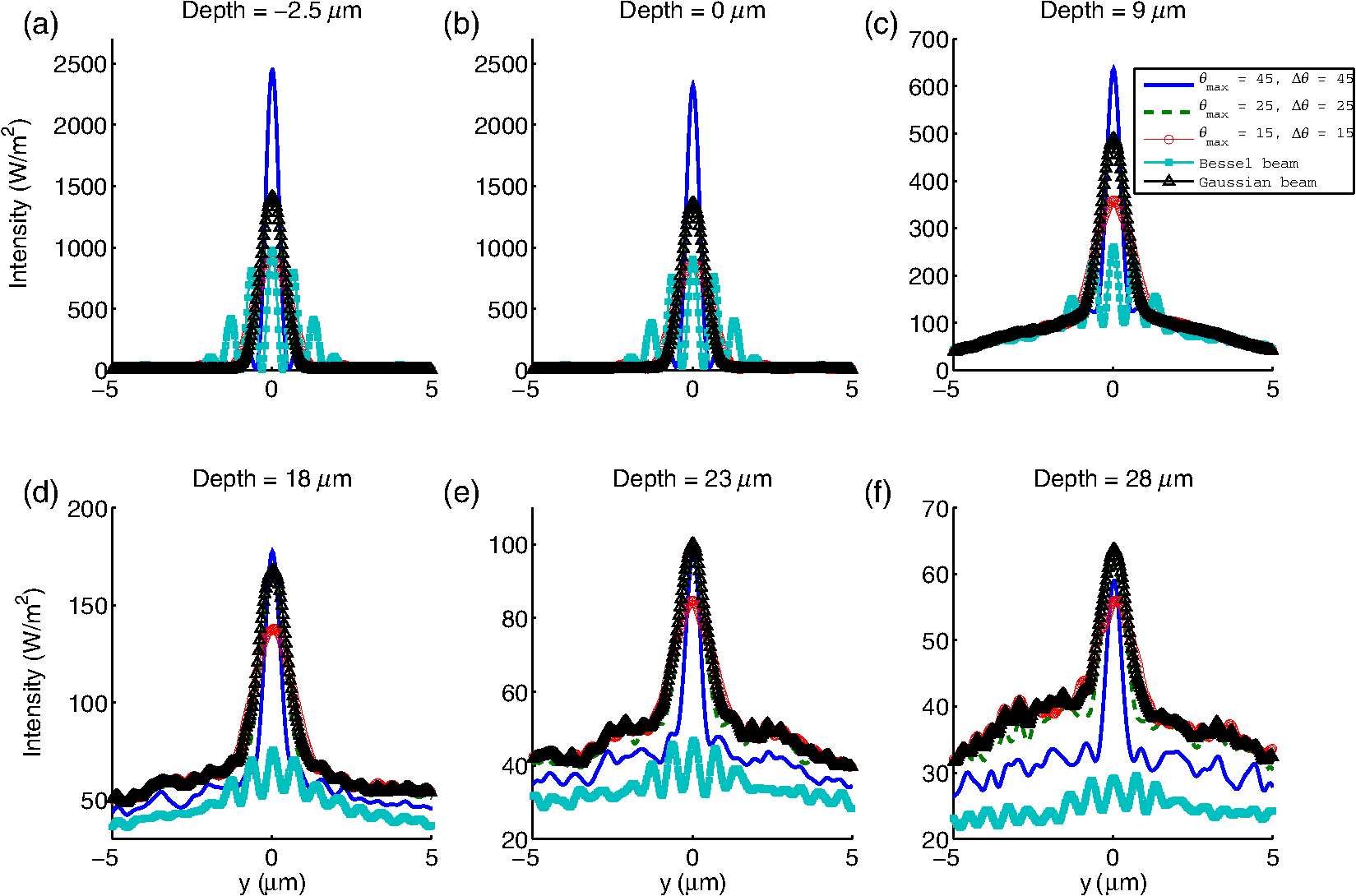
1.

Introduction

Focusing light deeply into scattering media is important in many research fields.^1–4 In biophotonics, it is used, e.g., for obtaining three-dimensional (3-D) microscopical pictures from tissue using established methods such as laser-scanning microscopy or multiphoton microscopy. There are several types of beams which are of particular interest due to their wide spread applications, e.g., a Gaussian beam,⁵ a Bessel beam,⁶ and a sinc-function type beam,⁷ which is called a focused beam within this manuscript. The Gauss beam is used in many fields of science since it models the fundamental laser mode (the lowest mode of an optical cavity).^5,8 A common application for the Bessel beam is light sheet microscopy.^9,10 Most of the studies done on the Bessel beam were either concentrating on the propagation of the beam itself in vacuo and the manipulation of its properties^6,11–13 or on the interaction between that beam and the scattering media. Those studies have been either experimental or used an approximated numerical solution such as the beam propagation method^14,15 (BPM). In this work, a quasi-Bessel beam is simulated in two-dimensions (2-D). This is different from a Bessel beam which cannot be simulated in 2-D due to the loss of the third dimension, which makes it impossible to use cylindrical symmetry. Finally, the focused beam, as it is called here, is interesting because it is obtained when an objective is over-illuminated by a homogeneous extended source (plane wave illumination) delivering a highly focused beam.^7,16,17

In previous works, numerical solutions of Maxwell’s equations were used to generate a focused beam by applying the angular spectrum of plane waves method (ASPW).^16–18 This solution proved to be adaptable to many beam profiles. For example, the Bessel beam was modeled using the ASPW, but was computed with the BPM.^9,10,19

In this work, the interaction between the incident light and the scattering media is examined for the different beam profiles using a numerical solution of Maxwell’s equations. It is shown that a less focused beam shows a similar performance compared to a highly focused one in delivering focused light deep into the scattering medium. The numerical simulations are performed using the finite-difference time-domain (FDTD) method. These simulations are carried out in 2-D due to the lower demand on the computational performance compared to calculations in 3-D. Moreover, in order to compare the penetration depth for each beam, the respective beam is scanned through the scattering media using a recently developed postprocessing method,¹⁷ which is also applied to smooth the interference effects.

2.

Theory

2.1.

ASPW Method

The ASPW approach is applied to model the light propagation of different focused beams. The ASPW describes the optical fields of the focused beams as a superposition of propagating plane waves.²⁰ In brief, first the spatial distribution of the electric field $E(x=0,y)$ in the focal plane is given. Then using a Fourier transform, the electric field versus spatial frequency $\widehat{E}(k_y)$ is calculated. By substituting the integrands in the Fourier transform, the angular description $\widehat{E}(\theta )$ in the far field is obtained.²¹ Following the work of Richards and Wolf, we model the focusing effect by the usage of an aplanatic lens. Thus, we need to take the geometric intensity law into account.⁷ After these mathematical manipulations, we write the spatial electric field as a function of the angular far field in a discretized form to facilitate the simulations later on using plane waves incident at discrete angles:

Eq. (1)

$$E(x,y)=\sum _{m=1}^M\widehat{E}({\theta }_m)\exp [jk(x\cos {\theta }_m+y\sin {\theta }_m)]\sqrt{\cos {\theta }_m},$$

where $M$ is the number of plane waves used to model the beam and ${\theta }_m$ is the incident angle for the $m$’th plane wave measured relative to the $x$-axis in the $x-y$ plane (see Fig. 1). The propagation direction in the 2-D case is the $x$-direction, whereas the $y$ denotes the lateral direction. The electric field in the $z$-dimension is constant making the power infinite. Thus, we normalize all beams to a given differential power. Another advantage of performing the investigation in 2-D is the decoupling of Maxwell’s equations into two sets of equations for two independent polarizations.²² In this study, we are concentrating on the parallel polarization ($E_x=E_y=0$). Therefore, all electric field components are polarized in the $z$-direction. Thus, the subscript is suppressed.

Fig. 1

Geometry of the simulations as carried out in this paper. The setup is infinite in $z$-direction. The electric field is propagating in the $x$ direction while being polarized in $z$-direction. The dark region in the middle of the beam is to visualize the focusing effect after going through the lens.

3.

Simulations

4.

Results

In Fig. 2, the intensity is shown when using a focused beam (${\theta }_{\max }=45\mathrm{deg}$) at different focus positions, whereas in Fig. 3, the same is shown for the quasi-Bessel beam case (${\theta }_{\max }=45\mathrm{deg}$, $\mathrm{\Delta }\theta =20\mathrm{deg}$). The two figures have been normalized to an incident differential power of $1\mathrm{W}/\mathrm{m}$ in each case. In both cases, the scatterers have a refractive index of $n_s=1.5$. It can be observed that certain transmission channels occur in the medium.²⁸

Fig. 2

The intensity ($\mathrm{W}/{\mathrm{m}}^2$) of a focused beam at different focus positions (${\theta }_{\max }=45\mathrm{deg}$). The upper left picture shows the scatterers in blue, while they are omitted in the other pictures for better visibility of the beam shape. The refractive indices are $n_m=1.33$, and $n_s=1.5$. $x_0$ is the focal position. (a) 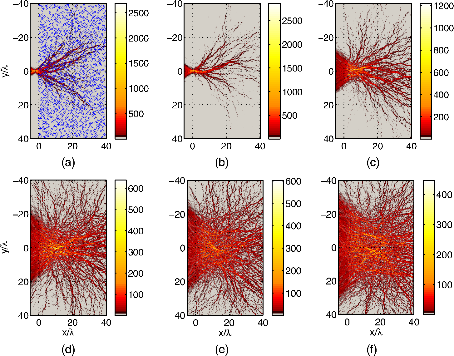$x_0/\lambda =-2.5$, (b) $x_0/\lambda =0$, (c) $x_0/\lambda =9$, (d) $x_0/\lambda =18$, (e) $x_0/\lambda =23$, and (f) $x_0/\lambda =28$.

Fig. 3

The intensity ($\mathrm{W}/{\mathrm{m}}^2$) of a quasi-Bessel beam at different focus positions (${\theta }_{\max }=45\mathrm{deg}$, $\mathrm{\Delta }\theta =20\mathrm{deg}$). The upper left picture shows the scatterers in blue, while they are omitted in the other pictures for better visibility of the beam shape. The origin in the longitudinal direction is placed at the starting point of the scatterers. The refractive indices are $n_m=1.33$, and $n_s=1.5$. $x_0$ is the focal position. (a) 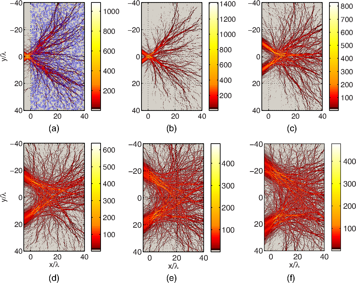$x_0/\lambda =-2.5$, (b) $x_0/\lambda =0$, (c) $x_0/\lambda =9$, (d) $x_0/\lambda =18$, (e) $x_0/\lambda =23$, and (f) $x_0/\lambda =28$.

The main problem at this point is that due to interference, it is difficult to get a quantitative comparison between the simulated beams while propagating through different scattering media. Averaging over multiple randomly chosen distributions of scatterers is a possible solution to obtain a smoother dependence of the intensity versus spatial position. However, this increases the simulation time. A more efficient solution is to use the ASPW method and to scan the beam as explained in the theory sections. Here, the focus is scanned in the lateral direction ($\pm 20\mu \mathrm{m}$). Then we average the intensity from all of these lateral scans incoherently to obtain the averaged intensity for each depth. As an example, the averaging of the intensity in Figs. 2 and 3 can be seen in Figs. 4 and 5, respectively. To further enhance the averaged results, 10 randomly chosen distributions of scatterers were applied in addition to the usage of the beam scanning.

Fig. 4

The intensity ($\mathrm{W}/{\mathrm{m}}^2$) for the focused beam in Fig. 2, averaged over a lateral range. $x_0$ is the focal position. (a) $x_0/\lambda =-2.5$, (b) $x_0/\lambda =0$, (c) $x_0/\lambda =9$, (d) $x_0/\lambda =18$, (e) $x_0/\lambda =23$, and (f) $x_0/\lambda =28$.

Fig. 5

The intensity ($\mathrm{W}/{\mathrm{m}}^2$) for the quasi-Bessel beam in Fig. 3, averaged over a lateral range. $x_0$ is the focal position. (a) 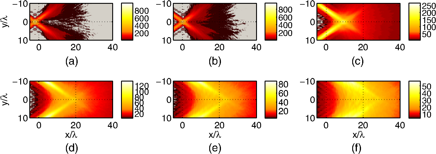$x_0/\lambda =-2.5$, (b) $x_0/\lambda =0$, (c) $x_0/\lambda =9$, (d) $x_0/\lambda =18$, (e) $x_0/\lambda =23$, and (f) $x_0/\lambda =28$.

In Fig. 6, the on-axis intensity is shown for all beams after being scanned through the scattering medium having $n_s=1.5$. It should be noted that the position of the maximal intensity of the beam $(x_0)$ is different from the position without scatterers (${\widehat{x}}_0$). Thus, a correction term considering the refractive indices of both the scatterers and the surrounding is used to get the approximate new position of the focus:

Fig. 6

The on-axis intensity for the focused, Gaussian, and quasi-Bessel beams for the same incident differential power. The refractive indices are $n_m=1.33$ and $n_s=1.5$.

Fig. 7

The lateral profile of the beams at different depths for $n_m=1.33$ and $n_s=1.5$. The differential power of each incident beam is equal to $1\mathrm{W}/\mathrm{m}$. The quasi-Bessel beam has ${\theta }_{\max }=45\mathrm{deg}$ and $\mathrm{\Delta }\theta =20\mathrm{deg}$, while the Gaussian beam has a $\mathrm{FWHM}=0.86\mu \mathrm{m}$. (a) $\mathrm{Depth}=-2.5\mu \mathrm{m}$, (b) $\mathrm{depth}=0\mu \mathrm{m}$, (c) $\mathrm{depth}=9\mu \mathrm{m}$, (d) $\mathrm{depth}=18\mu \mathrm{m}$, (e) $\mathrm{depth}=23\mu \mathrm{m}$, and (f) $\mathrm{depth}=28\mu \mathrm{m}$.

Fig. 8

The on-axis intensity for the beams using two sizes of cylindrical scatterers ($d=1\mu \mathrm{m}$ for symbols with lines and $2\mu \mathrm{m}$ for symbols only) while $n_s$ is kept equal to 1.45.

5.

Discussion

Obviously, for a given distribution of the scatterers, the penetration depth depends mainly on the scattering properties of the considered medium. However, it is interesting to note that the rate of change of the transmission channels seen in Figs. 2 and 3 depends heavily on the type of beam. For the focused beam (Fig. 2), a shift of $1\mu \mathrm{m}$ ($x_{\mathrm{sh}}=1\mu \mathrm{m}$) is enough to change the transmission channels considerably (not shown). In the case of the quasi-Bessel beam on the other hand (Fig. 3), the focus can be shifted by $10\mu \mathrm{m}$ and still mostly retain the same transmission channels. After the incoherent averaging in Figs. 4 and 5, it is easier to study the decrease of the beam intensity versus depth. Furthermore, the channels that could be seen before in Figs. 2 and 3 disappear. This indicates, as expected, that such channels depend on the individual distribution of the scatterers.

By adding the intensity of the two beams corresponding to the angular ranges of $|\theta |=[0\mathrm{deg}:25\mathrm{deg}]$ and $|\theta |=[25\mathrm{deg}:45\mathrm{deg}]$ in Fig. 6, we observe that it is approximately equal to the intensity of the beam in the range of $|\theta |=[0\mathrm{deg}:45\mathrm{deg}]$ at the surface of the sample. This is due to the fact that each beam is normalized to the same incident differential power, and for the beam in the range of $|\theta |=[0\mathrm{deg}:45\mathrm{deg}]$, we get about double the intensity of the arithmetic mean of the two beams in the ranges of $|\theta |=[0\mathrm{deg}:25\mathrm{deg}]$ and $|\theta |=[25\mathrm{deg}:45\mathrm{deg}]$ because of the coherent addition of the plane waves. By going deeper into the sample, the light experiences more scattering interactions and less constructive interference occurs in the focal region due to the decreasing nonscattered part of the light. As a result, we find that the intensity of the beam in the range of $|\theta |=[0\mathrm{deg}:45\mathrm{deg}]$ equals the arithmetic mean of the intensities of the beams in the ranges of $|\theta |=[0\mathrm{deg}:25\mathrm{deg}]$ and $|\theta |=[25\mathrm{deg}:45\mathrm{deg}]$.

Usually, a beam with a larger maximum divergence angle has a tighter focus. Since all the simulated beams have the same incident differential power, the more focused beam has higher intensity at the focus. This can be seen in, e.g., Fig. 7 at the depth of $-2.5\mu \mathrm{m}$. This changes when the beams propagate through the scattering medium. At higher depths, the high numerical aperture (NA) beams lose their advantage of having higher intensity at the focus to some extent. This can be visualized by looking at the propagation path of the individual plane waves that make up these beams. For the focused beam with ${\theta }_{\max }=45\mathrm{deg}$, the most divergent plane waves propagate a longer distance in the scattering medium due to their more oblique propagation directions and thus, they are more attenuated and comparable to the plane waves which are incident at smaller angles. This also explains the good performance of the Gaussian beam, which has most of its power in the small angles, while the quasi-Bessel beam shows a disadvantage in this case since relatively large angles are applied. In addition, using low NA beams proves more efficient because it avoids the unnecessary illumination of the sample with the light coming from the large incident angles, which prevents, e.g., bleaching in biological samples. We note that it is not so common to have a Bessel beam which is strongly focused, since the most attractive feature of such a beam is the large depth of field.¹⁰ However, our purpose here is to examine the basics of the propagation of such a beam. Also, since we are only simulating in 2-D, we do not have the option of simulating a real Bessel beam since it will simply appear as a sinusoidal wave.

As can be seen in Fig. 7, the intensity at $y$-values outside the beam focus area keeps rising at different rates for each of the simulated beams when the focus depth is increased. This “background” intensity is caused by multiple scattered light. Thus, it also affects the decrease rate of the curves in Fig. 6 making it difficult to judge where and if the intensity curves of different beams, which are only due to the nonscattered light, intersect.

In order to study only the nonscattered contribution to the intensity at the focus area versus depth, the following analytical equation was applied:

In Eq. (7), a Beer–Lambert exponential term is added to the ASPW expression of Eq. (1) to take into account the decrease in intensity due to scattering in a medium with a certain ${\mu }_s$.

We validated this model by comparing its results to those obtained with the FDTD method. Three more FDTD simulations were run ($n_s=1.4,1.5$, and 1.9 in $n_m=1.33$ corresponding to $\rho =117$, 19.8, and $3.4\mu \mathrm{m}$, respectively) using a lower volume concentration of 5% for cylinders with diameter of 1 μm. This was done to decrease the influence of the dependent scattering. The analytical model shows good agreement to the FDTD simulations at low scattering ($\rho =117$ and $19.8\mu \mathrm{m}$). For the higher scattering ($\rho =3.4\mu \mathrm{m}$), the curves started showing significant differences due to dependent scattering. The beams profile at three different depths calculated with Eq. (7) can be seen in Fig. 9 for similar scattering parameters as in Fig. 7 ($\rho =3.84\mu \mathrm{m}$) but for a lower concentration ($\mathrm{conc.}=-5\%$). As an advantage of using this model, we can investigate the focus due to the nonscattered light much deeper in the scattering medium than is possible with the FDTD method, compare to Fig. 7. From Fig. 9, we can see that the deeper the focus depth, the more the widths of the beams are broadening and the more the profiles of the different beams approache each other as expected from Fig. 7. This is due to the smaller contribution of the plane waves incident at larger angles. Figure 10 shows the intensity ratio of the beams with ${\theta }_{\max }$ of 25 deg to ${\theta }_{\max }$ of 45 deg for the same scattering medium. It can be seen that for depths larger than $25.7\mu \mathrm{m}$, the intensity of the smaller NA beam is larger than that for the larger NA beam. Thus, at large depths not only the total intensity at the focus position is larger for smaller ${\theta }_{\max }$ compared to larger ${\theta }_{\max }$ but also the intensity due to nonscattered light. Figure 10 shows, in addition, the intensity ratio of the focused beams with ${\theta }_{\max }$ of 35 deg to ${\theta }_{\max }$ of 70 deg. In this case, for depths larger than about $8\mu \mathrm{m}$, the nonscattered intensity of the smaller NA beam is larger than that of the larger NA beam. We note that a maximal incident angle of 70 deg corresponds to very high NA objective used in practice.¹

Fig. 9

Beam profiles at three different depths using the analytical solution for the nonscattered light ($\rho =3.4\mu \mathrm{m}$).

Fig. 10

Ratio of the intensities for different beams using the analytical solution for the nonscattered light for the case when $\rho$ is equal to 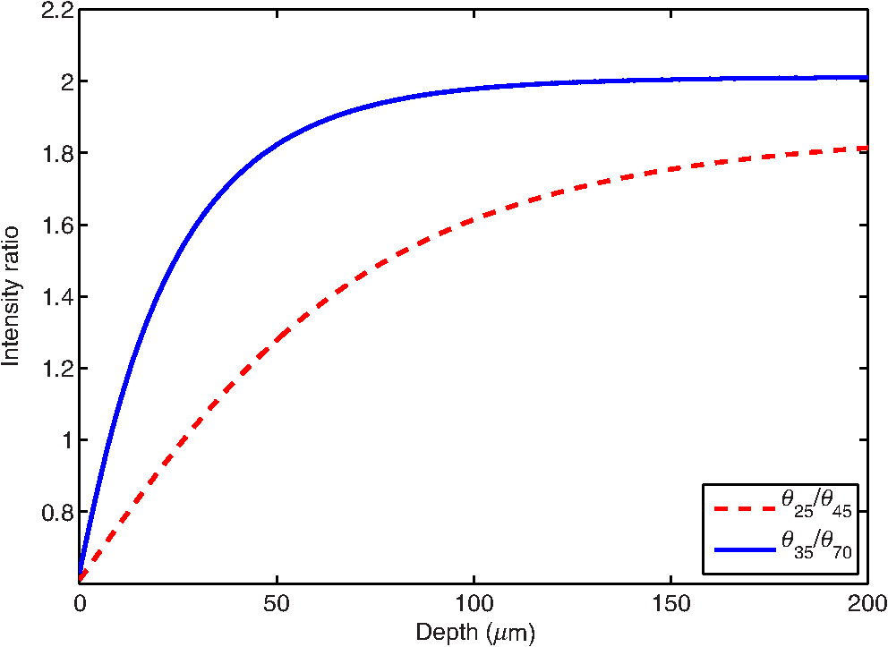$3.4\mu \mathrm{m}$.

Due to the large hardware resources needed for the FDTD method, we simulated the light propagation only in a relative small area. Therefore, we used scattering objects which have large scattering coefficients. This restriction can be released when the analytical equation is used allowing the use of more realistic optical properties for biomedical tissues. Thus, using a typical scattering coefficient which is, e.g., 10 times lower than is applied in Fig. 10, it follows that the shown curves are also scaled by a factor of 10. This means that the depths, where the intensity ratio is 1, are also a factor of 10 larger. For example, it follows that the intensity of the nonscattered light of a relative low NA beam with ${\theta }_{\max }$ of 35 deg is larger than that of a high NA beam with ${\theta }_{\max }$ of 70 deg for depths larger than about $80\mu \mathrm{m}$. However, we also note that the depth where the lateral profiles of the beam approach each other is increased (in the above case at about $800\mu \mathrm{m}$).

The previously mentioned conclusions that came from applying Eq. (7) can be generalized to the 3-D case. However, special care needs to be taken by adding an extra vector to the equation to control the polarization of the beam.²⁵ Figure 11 shows the 3-D results corresponding to the 2-D results shown in Fig. 10. It is interesting to note that we see the same phenomena of intensity enhancement when using a low NA beam in comparison to the high NA case. Of course, it should be noted that in this case, we have to consider solid angles since we are dealing with the 3-D setup. This is the reason for the higher intensity enhancement found in Fig. 11 when compared to Fig. 10 despite having the same ratio between the divergence angles in both cases.

Fig. 11

Ratio of the intensities for different beams using the analytical solution for the nonscattered light for the case when $\rho$ is equal to $3.4\mu \mathrm{m}$ in 3-D.

As a rule of thumb, the scattering cross section increases with the size of the scatterer.²⁷ This can be seen in Fig. 8, where the on-axis intensity for the larger scatterers ($d=2\mu \mathrm{m}$) decreases at a higher rate than the case of smaller scatterers ($d=1\mu \mathrm{m}$). This also agrees with the analytical solution of the scattering of a plane wave by a cylinder²⁷ since for the bigger cylinder ($d=2\mu \mathrm{m}$), we obtain a scattering cross section $C_{\mathrm{scat}}$ of $2.7\mu \mathrm{m}$, whereas for the smaller cylinder ($d=1\mu \mathrm{m}$), $C_{\mathrm{scat}}$ is $0.39\mu \mathrm{m}$. Comparing the results presented in Fig. 8, it can be seen that the efficiency of the averaging is worse for the cylinders with a larger diameter. This is mainly because of the higher correlation of the results obtained in the case of the larger scattering objects due to the smaller ratio of the lateral beam shifts to the cylinder diameter.

6.

Conclusion

In this study, the propagation of several types of beams through scattering materials was investigated. Focused, Gaussian, and quasi-Bessel beams were simulated in 2-D. The study was performed by numerically solving Maxwell’s equations using the FDTD method. Solutions of Maxwell’s equations are superior to Monte Carlo simulations because all effects of classical physics such as dependent scattering are included.²⁹ The incident beams were modeled using the ASPW method, which enables the manipulation of the phases of the individual plane waves that constitute the modeled beam. The simulation of the scanning of the beams is achieved in an efficient way¹⁷ both in the axial direction (to study the effect of depth scanning on the quality of the beam focus) and in the lateral direction (which allows for an effective averaging technique).

The results show that for focusing light in scattering media, the focus intensity of a high NA beam decreases faster versus depth than is the case for a small NA beam. The FDTD simulations demonstrate that at a certain depth in the scattering medium, the total intensity at the focus position (including both the nonscattered and the scattered light) is larger, e.g., for the ${\theta }_{\max }=25\mathrm{deg}$ focused beam compared to the ${\theta }_{\max }=45\mathrm{deg}$ focused beam. However, due to the high amount of necessary calculation time (for large depths and, thus, large simulation areas), the FDTD simulations do not show if this is also the case for the focus intensity of the nonscattered light, which is the important quantity for many microscopical applications. Here, we used a simple mathematical model to calculate the intensity profile for the nonscattered light versus depth and lateral positions. It shows that for large depths, the focus intensity of the nonscattered light is larger for the low NA beam than for the high NA one, e.g., about twice as large for the ${\theta }_{\max }=25\mathrm{deg}$ focused beam compared to the ${\theta }_{\max }=45\mathrm{deg}$ focused beam. In addition, we showed that for a large focus depth, the lateral profile of the nonscattered intensity of the low NA beams approaches that of the high NA beams resulting in a similar resolution when used in a microscope.

In summary, for microscopical applications deep in a scattering medium, the use of beams with a lower NA can be advantageous compared to higher NA beams. Finally, we note that the models used in this study can be readily extended from the 2-D to the 3-D case, where it is expected that the advantages of the low NA beams are even greater.