1.

Introduction

Both implementations of the spectral or Fourier domain optical coherence tomography (OCT), spectrometer based OCT and swept source OCT, can be used to produce cross-sectional (B-scan) images with high speed and high sensitivity. We will refer to spectral/Fourier or spectrometer based or swept source based implementations as spectral domain (SD) from now on for simplicity. Traditionally, in order to produce a B-scan, in both implementations, each channeled spectrum acquired while scanning the probing beam over the sample is subject to a fast Fourier transform (FFT). However, before the FFT, several preparatory signal processing steps are necessary, such as zero padding, spectral shaping, apodization, dispersion compensation, or data resampling. Without these preparatory steps, axial resolution and sensitivity suffer.¹ As all these steps can only be sequentially executed, the production of the B-scan images in real-time is limited. So far, several techniques involving both hardware and/or software solutions have been demonstrated to successfully eliminate or diminish the execution time of the preparatory steps. Correct resampling and compensation for dispersion mismatch are extremely important as an incorrect k-mapping or dispersion left unbalanced in the system broadens the coherence peak.² To eliminate the resampling step in spectrometer based OCT, a solution using a prism after the diffraction grating was proposed.³ However, this complicates the optics hardware, requires careful adjustment, and introduces losses. In swept source OCT, the swept sources are often equipped with a supplementary clock signal (k-clock)⁴ that not only adds to the cost of the source, but also requires a specialized, more sophisticated digitizer that in the end does not yield a perfect resampling and also limits the axial range of the image.⁵ Other techniques such as using an additional light source that produces several spectral lines in the region of interest of the spectrometer,⁶ parametric iteration methods,⁶ phase linearization techniques,^7,8 and automatic calibrations⁹ have been proposed. All these methods are normally computationally expensive and limit the real-time operation of OCT systems.

Dispersion compensation is another important limiting factor in obtaining high-resolution SD-OCT images. Both hardware and software (numerical) methods have been implemented to overcome this limitation.¹⁰ Compared to hardware methods, which involve physically matching the dispersion of the reference and the sample arms, the numerical dispersion compensation is more cost-effective and flexible. Various numerical techniques to compensate for dispersion, such as autofocusing,^10,11 have been developed. However, all the numerical algorithms used to compensate for dispersion involve Hilbert transformations, phase corrections, filtering, etc.; hence, a heavy computational loading and, therefore, numerical dispersion compensation has to be performed as a postprocessing step.

As the computational requirements for high-speed SD-OCT image processing usually exceed the capabilities of most computers, the display rates of B-scan images rarely match the acquisition rates for most devices. After the preparatory steps, most image analysis and diagnosis become a postprocessing operation. A true real-time (TRT) display of processed SD-OCT images when a B-scan is produced in the next frame time could vastly benefit applications that require instant feedback of image information, such as image guided surgery or endoscopy,¹² or ophthalmology, where it could aid with patient alignment and reduce session time.¹³ TRT display is also a prerequisite for three-dimensional (3-D) real-time imaging.¹⁴

Solutions involving parallel computing hardware enable dramatic increases in performance, taking advantage of devices such as graphics processing units (GPUs) or field-programmable gate arrays (FPGAs). By significantly reducing the computation time of preparatory steps, true real-time production of B-scan images becomes possible. However, as some of the preliminary steps are often based on iterative calculations, errors in correctly preparing the data are unavoidable.

In MS-OCT, where the FFT is replaced by cross-correlation, some of the preparatory steps (resampling and compensation for dispersion mismatch between the two arms of the interferometer) are no longer necessary.^15–17 Thus, the MS-OCT, being based only on mathematical operations, is able, in principle, to produce better images in terms of their axial resolution and sensitivity than their FFT-based counterparts. Moreover, as MS-OCT involves mathematical operations that can be performed in parallel, it makes sense to take advantage of tools already harnessed by the OCT community to produce images fast, such as GPU (Refs. 1819.20.21.22.23.24.25.–26) or FPGA (Refs. 2728.29.–30) hardware. In terms of computation speed, GPU is an efficient computational engine for very large data sets. By contrast, the FPGA can be as efficient as the GPU for large data sets, but FPGAs are better suited for applications where the size of the data to be processed is small.³¹ However, on FPGAs, memory is a scarce resource as the block RAM capacity of the FPGA is generally limited. In addition, when performing cross-correlations, which are required by the MS method, data from both the current channeled spectrum and the mask must be available simultaneously as both have to be loaded from the memory in the same clock cycle, which makes the FPGA solution highly dependent on fast memory operations. This favors GPUs as the technology of choice, instead of the FPGAs, to produce TRT MS based B-scan images. Apart from the superiority of the GPU in terms of memory availability, the developers should also consider in their choice that in the foreseeable future, the multicore architecture of the CPU and the many-core architecture of the GPU are likely to merge. This trend can be seen in the introduction of computing parallel solutions used as coprocessors, such as Intel Xeon Phi and NVIDIA Tesla. Visual Studio (Windows) and GCC (Linux) both offer programming environment and language support for these architectures. A GPU combines both fine-grained (threads) and coarse-grained (blocks) parallel architectures. This feature offers an optimal mapping for the specific structure of the signal generated by the OCT systems, where data points are processed by parallel threads and spectra are processed by thread blocks. In addition, the GPU is financially and technologically a more accessible solution. Finally, there are some other immediate benefits of using GPUs over FPGAs in OCT, such as no need for extra hardware (standard PC components are sufficient), availability of a free programming environment, language support, and additional libraries (NVIDIA CUDA C, CUDA FFT).

2.

Methodology of Producing MS Based B-Scans

In SD-OCT, a cross sectional image is produced by assembling A-scans (longitudinal reflectivity profiles) into a B-scan, with each A-scan being the result of a single FFT operation. For simplicity, let us consider that no preparatory steps are required before FFT. In this case, mathematically, we can describe a B-scan image as

In Eq. (1), ${\mathrm{CS}}_1,{\mathrm{CS}}_2,\dots {\mathrm{CS}}_r$ are channeled spectra collected at $r$ lateral positions (pixels along a line perpendicular to the axis connecting the system with the object) of the scanning beam on the sample, while $A_1,A_2,\dots A_r$ are their corresponding A-scans. All the $q$ components of a particular $i$ A-scan ($A_{i,1},A_{i,2},\dots A_{i,q}$) from lateral pixel $i$ are obtained simultaneously by a single FFT operation [$q$ is, in principle, equal to half the number of sampling points of each channeled spectrum ${\mathrm{CS}}_i(i=1\dots r)$, but very often, in practice, $q$ is increased by zero padding]. To obtain a B-scan image of size $r\times q$, a number of $r$ independent FFT operations need to be performed. As these operations can be executed in parallel, theoretically, the time to produce a B-scan image can be reduced to the time to perform a single FFT operation. In this case, the maximum time to deliver a B-scan, $T_{\mathrm{B}}(\mathrm{FFT})$, is made of the time to acquire all $r$ channeled spectra ${\mathrm{CS}}_i$ plus the processing time, which, using parallel processing, can be reduced to the time for a single FFT.

To keep the comparison of different regimes of operation simple, let us consider that the acquisition and processing are not interleaved.

As explained in Ref. 17, in MS-OCT, it is possible to generate B-scan images in two ways: by assembling A-scans as in conventional SD-OCT and also by assembling T-scans (transversal reflectivity profiles). Each component of the A-scan (or T-scan) is obtained by integrating the result of the cross-correlation between a channeled spectrum ${\mathrm{CS}}_i$ and a reference channeled spectrum (denoted from now on as mask) $M_j(j=1\dots p)$, recorded for an optical path difference (${\mathrm{OPD}}_j$) between the sample and reference arms of the interferometer when a highly reflective mirror is used as an object.

The integration is done over a window of size $W=2w-1$ points around the maximum value of the correlation result. The masks should be recorded at OPD values in the set ${\mathrm{OPD}}_1,{\mathrm{OPD}}_2,\dots {\mathrm{OPD}}_p$, separated by half the coherence length of the source or denser. To obtain a B-scan image of the same size as that obtainable in SD-OCT, a number of $p=q$ masks need to be recorded. In a matrix representation, an MS-based image can be presented as

Each column of the bidimensional array in Eq. (4) represents a T-scan, while each row contains the information to assemble an A-scan. As all the elements of this matrix can be computed independently, the time to produce, for example, an A-scan based B-scan can, in principle, be reduced to the time to perform a single cross-correlation.

In the equation above, $i$ is the lateral pixel index, $j=1\dots p$ signifies the depth, $i\mathrm{FFT}$ denotes the inverse fast Fourier transform, while the * operator is the complex conjugate. As suggested in a previous report,¹⁷ to speed up the process, instead of recording the values of the masks $M_j$, the $\mathrm{FFT}{(M_j)}^{*}$ values are precomputed and recorded instead. This reduces the time to work out the reflectivity $A_{ij}$ of a point in the A-scan to the time to sequentially execute two FFTs. To obtain a B-scan image of size $r\times p$, a number of $r\times p$ independent cross-correlations have to be performed. As these operations can be executed in parallel, the time to produce an MS-based B-scan image, $T_{\mathrm{B}}(\mathrm{MS})$, can, in principle, be reduced to the time to perform a single cross-correlation.

For a spectrum acquisition in $10\mu \mathrm{s}$, considering $r=200$ lateral pixels, $t_{\mathrm{acq}}=2\mathrm{ms}$. The time for a single FFT in the SD-OCT and for two FFT processes in the MS-OCT case can be absorbed into the acquisition time, as they are below a couple of microseconds. This means that $T_{\mathrm{B}}(\mathrm{MS})\approx T_{\mathrm{B}}(\mathrm{FFT})$.

As a consequence of the above analysis, it appears that it is possible to produce MS-based B-scan images at a rate similar to that of producing FFT-based B-scans.

In case data in the SD-OCT need to be prepared before FFT, then the processing time exceeds the time for a single FFT operation. Depending on the processing involved, which also depends on the nonlinearities to be corrected, the evaluation of a single A-scan via linearization/calibration followed by an FFT may exceed the time for $p$ correlations (considering implementation in parallel in the time for a single correlation in our discussion).

As these extra processes are not needed in MS-OCT, MS based B-scan images can then be produced at similar rates with, or even faster than, the FFT based method.

In all this discussion and in Eq. (6), we did not consider the time to transfer data between hardware components or between memories, therefore, in practice, $T_{\mathrm{B}}(\mathrm{MS})$ includes more terms than shown in Eq. (6). This means that MS-OCT cannot be faster than SD-OCT in producing a B-scan OCT image when no linearization/calibration is performed.

However, B-scans can still be produced in a TRT regime using the MS-OCT method.

3.

GPU Implementation and Experimental Setup

The MS principle can be applied to any SD-OCT technology. This is illustrated here on a conventional swept source OCT setup. The experimental setup employed for this paper is identical to that used in Ref. 15. Figure 1 illustrates the flow of data and the structure of trigger/clock signals required to produce a B-scan image.

Fig. 1

Overall structure of the graphics processing unit (GPU) enhanced optical coherence tomography (OCT) system illustrating the operation required for the production of a [master-slave (MS) or fast Fourier transform (FFT) based] B-scan image. DAQ, data acquistion board; SX, galvo-scanner; SS, swept source; BPD, balanced photodetector; DLL, dynamic link library.

A LabVIEW project is created to perform most of the tasks in the system. The choice for a LabVIEW implementation is dictated by its versatility, covering acquisition, processing, and visualization of data. LabVIEW is also highly popular among OCT research groups.^19,28,30 It facilitates easy interaction with the hardware via data acquisition (DAQ) boards and acquisition of data via digitizers or image acquisition (IMAQ) boards. This platform offers an excellent user interface and, in terms of development time, is superior to any C/C++ implementation. Our LabVIEW application generates a triangular waveform via the DAQ (NI PCI 6110) to drive the galvo-scanner (SX), acquires and stores the data into a buffer via a fast digitizer (Alazartech, Quebec, Canada, model ATS9350) according to timings set by the DAQ and the trigger signal provided by the swept source (SS, Axsun Technologies, Billerica, Massachusetts) and, finally, communicates with a GPU application via a dynamic link library (DLL). The GPU application performs the signal processing and generates the resulting image using OpenGL drawing primitives. The DLL and the GPU application exchange the buffered data as well as a number of control values required to manipulate the contrast and brightness of the image or the value of the window $W$ over which the correlation signal is integrated. The use of a standalone application that facilitates the LabVIEW project to communicate with CUDA code is not unique. The DLL could encapsulate the CUDA code (CUDA kernels). However, in this case, there are two main issues: (1) the GPU context needs to be created every time the DLL is called, which significantly increases the processing time and prevents the system from working in real time and (2) the DLL cannot load OpenGL to display the processed images.³²

For our experiments, a commonly available NVIDIA GeForce GTX 780 Ti (3 GiB on-board memory, 2880 CUDA cores) is used, installed in a Dell Precision 7500 equipped with dual CPUs (E5503, 4 cores @ 2.0 GHz).

To make a fair comparison between the MS and FFT methods, the internal clock signal equipping the swept source was used to sample the data, though it is not necessary for the MS-OCT method. According to the laser manufacturer, the maximum frequency of the clock signal is $\sim 330\mathrm{MHz}$, and the duty cycle of the laser emission is 45%, so for a sweeping rate of 100 kHz, a maximum of 1531 sampling points can be used to digitize each channeled spectrum. In practice, as the digitizer requires a number of data points evenly divisible by 32, 1472 sampling points are employed to digitize the entire spectral range of each channeled spectrum, which can be used to sample up to 736 cycles.

A number of $r=500$ A-scans are used to build each cross-sectional image; hence, a maximum image size of $500\times 736{\text{pixels}}^2$ could be produced at a frequency of $F_x=100\mathrm{Hz}$, while the galvo-scanner is driven with a triangular waveform at 500 Hz. In this way, the data acquisition time of a single frame (B-scan) is 5 ms. The time to buffer the necessary data to produce a B-scan image is depicted as process A in Fig. 2.

Fig. 2

Flow chart showing the timing of data acquisition (A), transfer (B), processing (C, D), and visualization (E, F) in a GPU enhanced OCT system. C and E refer to the spectral domain OCT method, and D and F to the MS-OCT method. The time intervals shown on the figure are compatible with true real-time operation of the system, practically obtained for 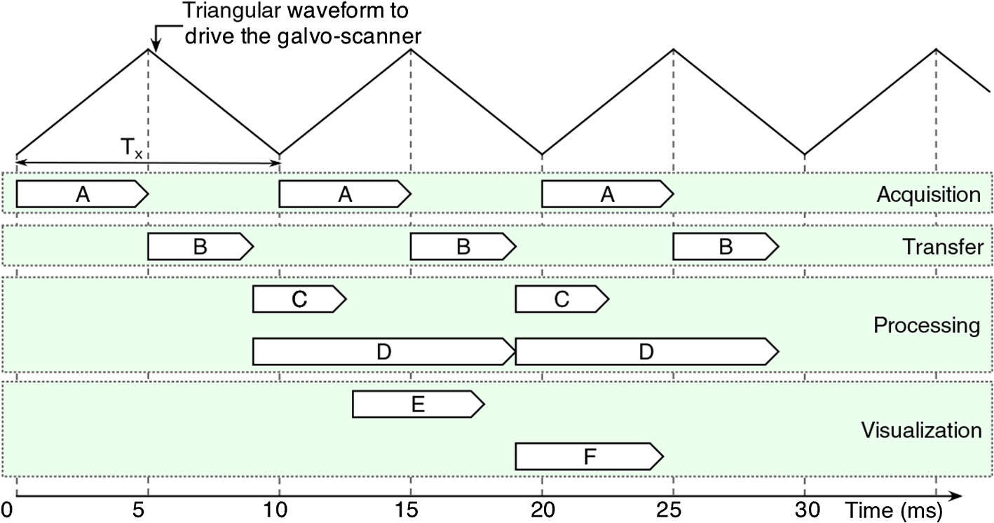$q=1024$ and $p=144$.

To ensure an acceptable real-time operation of the system, the data processing time required to produce the final B-scan image has to be $<10\mathrm{ms}$. In a conventional non-GPU enhanced application, after the acquisition of each buffer, data are directly accessed and processed by the CPU. The processing of data on the GPU is obviously faster than on the CPU; however, as the acquired data are not directly accessible by the GPU, the time to transfer data to the CPU memory (shared memory) accessible by the GPU has to be taken into account (process B in Fig. 2). Once in the shared memory, data can be processed either traditionally via FFTs (process C in Fig. 2) or using the MS method (process D). After processing, data are available to OpenGL for image generation and visualization (process E or F in Fig. 2 for displaying FFT or MS based B-scans, respectively).

To ensure a TRT operation of the system, the time to transfer data to the shared memory has to be less than the acquisition time (5 ms in our case), while the time allocated to processing or visualization has to be less than the period of the galvo-scanner (10 ms).

In Fig. 3, the entire chain of processes and operations required to display an image is presented. This chain starts from the moment data are available in the shared memory to be accessed by the GPU application for both FFT (A) and MS-OCT (B) methods. The simplest FFT based case is considered, where there is no need for dispersion compensation and no need for resampling of data. Processes C1 and D1 designate the transfer of data from the shared memory to the GPU memory. As the same amount of data is transferred in both C1 and D1 cases, it is expected that they take the same amount of time: $T_{\mathrm{C}1}=T_{\mathrm{D}1}$. Processes C6 and D6 designate the transfer of data from the GPU memory back to the local CPU memory (of the GPU application). In this case, as typically $p\ne r$, it is expected that $T_{\mathrm{C}6}=T_{\mathrm{D}6}$. Finally, C7 and D7 refer to the transfer of data to the OpenGL primitives for image generation and display.

Fig. 3

GPU threads execution in FFT-based OCT (A) and MS-OCT (B). C1 and D1 signify the process of data transfer from the shared memory to the GPU memory, C6 and D6 represent the transfer of data from the GPU memory back to the local CPU memory, and C7 and D7 represent data transfer to OpenGL for image generation and visualization.

4.

Results

In order to establish the conditions to produce TRT based B-scan images, the time required for process B shown in Fig. 2, as well as the time required for the components of Fig. 3 are measured. Once the best settings that ensure a (true) real-time operation are established, in vivo images of the human eye are produced.

4.2.

Fast B-Scan Imaging

Ethical approval to image researchers’ retinas was obtained from the Faculty of Sciences at University of Kent ethics committee, application “Tests of optical instruments for imaging the eye, assembled by the Applied Optics Group (AOG), on AOG researchers.” The images were collected from the eyes of two of the authors, Adrian Bradu and Adrian Podoleanu. Both coauthors have signed consent forms. In this manuscript, only images from AB’s eye are presented.

The capability of the system to produce MS based B-scan images sufficiently fast, of comparable resolution and sensitivity as their FFT based counterpart, is demonstrated by two movies (Videos 1 and 2) showing B-scans side by side using both methods. Figures 4 and 5 show in vivo B-scan images of the human fovea and optic nerve area, respectively, obtained using the two methods (frames from the generated videos). To produce both images, $q=1024$ sampling points for each channeled spectrum are used, resulting in $7.2\mu \mathrm{m}$ depth between consecutive points in the FFT based A-scan. As a consequence, $p=384$ masks separated by $7.2\mu \mathrm{m}$ are recorded in order to obtain a nearly perfect axial correspondence between the horizontal lines of the two images. As illustrated in Table 1, in this case, TRT is not achieved (the time to produce an MS based B-scan image is 21.9 ms, longer than $T_x$). Therefore, although both MS and FFT based B-scans are produced simultaneously, and the images in the movies are displayed at a rate close to that demanded to display the MS based images only.

Fig. 4

B-scan images of size $500(\text{lateral})\times 384(\text{axial}){\text{pixels}}^2$ of the optic nerve area of AB showing lamina cribrosa obtained using the conventional Fourier domain technique (left) and the MS method (right). The axial size of images is evaluated in air. The images are extracted from a movie (Video 1) produced in real time ($\sim 50\mathrm{fps}$) (MOV, 14.6 MB) [URI: http://dx.doi.org/10.1117/1.JBO.20.7.076008.1].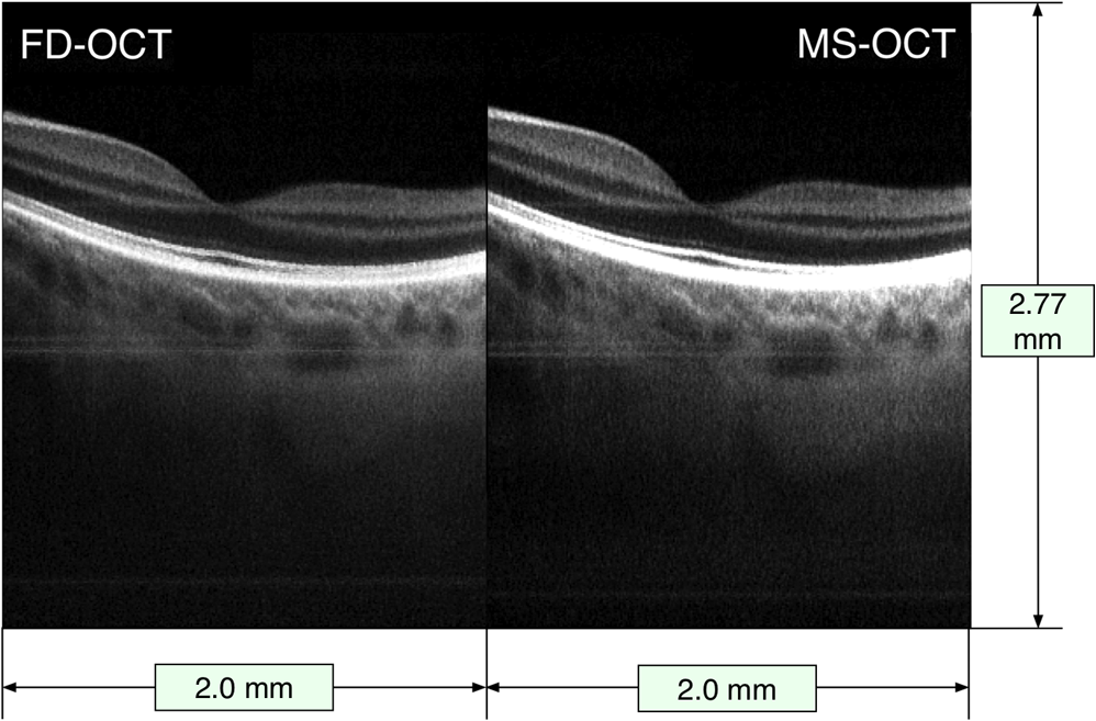

Fig. 5

B-scan images of size $500(\text{lateral})\times 384(\text{axial}){\text{pixels}}^2$ of the foveal area of AB obtained using the conventional FFT-based technique (left) and the MS method (right). The lateral size of images is evaluated in air. The images are extracted from a movie (Video 2) produced in real time ($\sim 50\mathrm{fps}$) (MOV, 14.4 MB) [URI: http://dx.doi.org/10.1117/1.JBO.20.7.076008.2].

The fact that the two images are not perfectly axially aligned can be seen better in the two movies (Videos 1 and 2) from which the images are extracted. There, it is easily observable that the horizontal lines (artifacts the movies are not corrected for) originate from slightly different depths in the two images. The FFT based image is cropped to cover a 384 points subset from each A-scan. To record the two movies, no fixation lamp was used. Also, no (post)processing step was applied to the images to correct for movements, and no image registration procedure was used. The only processing operation applied to the images was a manual adjustment of the contrast and brightness, which explains the small difference between the gray levels in the movies shown side by side. The movies are displayed in real time at $\sim 50\mathrm{fps}$. To produce the images in Figs. 4 and 5, the frames of the movies are corrected for movement before averaging 25 consecutive B-scans. It is obvious that the images produced by MS are similar in terms of contrast and resolution with those produced by conventional SD-OCT. To produce the movies, the optical power at the cornea was limited to 2.2 mW, below the ANSI (Ref. 33) maximum allowed level for the 1060-nm region.

5.

Conclusion

Fast display of MS based B-scan OCT imaging is demonstrated by harnessing the GPU capabilities to perform the entire signal processing load that the MS method requires. While the MS method exhibits sensitivity and axial resolution similar to that provided by the FFT based technique, for the particular GPU used in this work, the production of the B-scan retinal images in a TRT regime is not possible due to the limited memory of the GPU. TRT imaging regime is achievable, however, for a reduced size of $500\times 144{\text{pixels}}^2$ for the B-scan images. The axial size of 144 pixels is not sufficient when imaging the retina. A GPU with a larger memory is necessary to increase the number of depths $p$ processed in parallel. However, an $\sim 50\mathrm{Hz}$ frame rate was achieved for the display of B-scans with 384 depths, showing that by harnessing the GPU cards, the bottleneck of the MS method in producing B-scans¹⁷ can be successfully addressed.

When the GPU application is neither computationally nor memory bounded, the TRT operation is secured. The GPU method proposed here is computationally and memory bounded. As specified in Table 1, for the MS case, a large number of sampling points such as $q=1472$ or $q=1280$ with $p=384$ masks require a memory size larger than that available. As soon as $q$ exceeds 1024, the GPU method becomes computationally bounded and a TRT operation cannot be ensured.

As demonstrated in previous studies,^15–17 the MS method is highly suitable for 3-D images. Each point $A_{ij}$ in the 3-D image is the result of a cross-correlation operation. Preferably, 3-D via the MS method would assemble $p$ en face images into a volume. As this report is about B-scans, let us consider a 3-D assembly of B-scans into a 3-D volume. As the swept source employed in the study sweeps at 100 kHz, considering a number of lateral pixels as in previous reports,^15,16 of $r=200$, a 3-D dataset of size $200\times 200\times 384{\text{pixels}}^3$ can be acquired in 0.4 s, while $p=384$ masks determine the number of axial points in the volume. Due to the limitations on the shape and frequency of the signal that can be sent to the galvo-scanners, the time to acquire data is $t_{\mathrm{acq}}=0.8\mathrm{s}$. As a consequence, to ensure a 3-D TRT operation of the system, once data are acquired, the $200\times 200\times 384{\text{pixels}}^3$ operations have to be produced within 0.8 s. For our hardware implementation, this is feasible, as the time to transfer data to the shared memory is evaluated as $<0.45\mathrm{s}$. However, especially due to the limited amount of memory available on the GPU, the TRT production of the full size 3-D images is not possible yet.

Operating the setup in the MS-OCT regime cannot deliver a B-scan as fast as its SD-OCT counterpart when no linearization is required, so the advantage of using the MS-OCT may not be apparent. However, if resampling of data is needed prior to FFT processing, or numerical calculations to eliminate the dispersion mismatch between the arms of the interferometer are required, then the balance swings in favor of the MS-OCT method. FFT-based B-scan images obtained with the clock disabled are not shown here. In such a case, they would display axial resolutions $>50\mu \mathrm{m}$ with a barely distinguishable definition at larger depths. The B-scan OCT images obtained using the MS-OCT look exactly the same as those generated with the conventional FFT-based method applied to linearized data. If, let us say, a swept source with no clock is employed, then a software linearization calibration procedure needs to be implemented. Such a procedure would extend the time for the FFT-based method by at least 50% while the correction may not be perfect at all depths. The images are not shown, as they have been already reported by other groups. The imperfections in linearization/calibration may swing the balance again in favor of the MS-OCT via GPU. Better GPUs with more memory that would allow production of larger image sizes are already available. Also, computers with faster interconnects can reduce the time to transfer data between different memories, improving both latency (data available to the GPU application sooner) and visualization throughput (at higher frame rates).

The time to produce an MS-based B-scan demonstrated here when considered in combination with other advantages in terms of hardware cost makes the MS-OCT method worth considering for imaging the eye. As there is no need for data resampling, MS-OCT can operate with a simpler swept source, not equipped with a k-clock, or even with potentially highly nonlinear tuneable lasers. An MS-OCT system can operate in terms of its axial resolution and sensitivity decay with depth at the level of a perfectly corrected SD-OCT setup. Therefore, MS-OCT has the potential to provide better sensitivity, resolution, and better axial range than practical systems implementing conventional FFT technology, which depart from perfectly corrected systems in terms of linearization and dispersion compensation.

With a speed in displaying B-scans comparable to those typically reported by SD-OCT systems, as detailed here, MS-OCT can become the technique of choice for TRT imaging in ophthalmology and other applications that require instant feedback, such as in surgery.