Modified multiscale sample entropy computation of laser speckle contrast images and comparison with the original multiscale entropy algorithm

Anne Humeau-Heurtier; Guillaume Mahé; Pierre Abraham

doi:10.1117/1.JBO.20.12.121302

28 July 2015 Modified multiscale sample entropy computation of laser speckle contrast images and comparison with the original multiscale entropy algorithm

Anne Humeau-Heurtier, Guillaume Mahé, Pierre Abraham

Author Affiliations +

Journal of Biomedical Optics, Vol. 20, Issue 12, 121302 (July 2015). https://doi.org/10.1117/1.JBO.20.12.121302

Abstract

Laser speckle contrast imaging (LSCI) enables a noninvasive monitoring of microvascular perfusion. Some studies have proposed to extract information from LSCI data through their multiscale entropy (MSE). However, for reaching a large range of scales, the original MSE algorithm may require long recordings for reliability. Recently, a novel approach to compute MSE with shorter data sets has been proposed: the short-time MSE (sMSE). Our goal is to apply, for the first time, the sMSE algorithm in LSCI data and to compare results with those given by the original MSE. Moreover, we apply the original MSE algorithm on data of different lengths and compare results with those given by longer recordings. For this purpose, synthetic signals and 192 LSCI regions of interest (ROIs) of different sizes are processed. Our results show that the sMSE algorithm is valid to compute the MSE of LSCI data. Moreover, with time series shorter than those initially proposed, the sMSE and original MSE algorithms give results with no statistical difference from those of the original MSE algorithm with longer data sets. The minimal acceptable length depends on the ROI size. Comparisons of MSE from healthy and pathological subjects can be performed with shorter data sets than those proposed until now.

1. Introduction

Optical medical imaging has found an increased interest for the monitoring of peripheral cardiovascular systems, such as the microvascular system. Among the optical medical imaging techniques that have emerged recently for the evaluation of the microvascular network, we find laser speckle contrast imaging (LSCI).¹^–⁴ LSCI is based on the wide-field illumination with a coherent light source of the tissue surface under study. Due to constructive and destructive interference coming from phase differences involved in the backscattered light, a speckle pattern is obtained on the detector. In LSCI, the resulting laser speckle pattern is imaged with a camera. Because some of the photons scatter dynamically from moving particles in the tissue, a decorrelation (blurring) of the laser speckle pattern is obtained on the camera. This blurring can be quantified by computing the speckle contrast $K$ as

Eq. (1)

K (x, y) = \frac{σ_{N}}{μ_{N}},

where

σ_{N}

and

μ_{N}

are, respectively, the standard deviation and mean of the pixel intensity in a neighborhood

N

around the pixel in the speckle raw data. The LSCI perfusion index is then computed from the contrast value: LSCI perfusion value is inversely proportional to the contrast

K

(see below). LSCI has the advantage of being a full-field noninvasive optical technique with no scanning procedure to capture the data and which gives images with high spatial and temporal resolutions.⁵^–⁸ Moreover, the optical system can be obtained with low-cost devices.⁹ LSCI is still the object of many studies and improvements.¹⁰^–¹⁵

Once medical images are acquired, the challenge is to extract relevant physiological information. This is often possible via the use of signal processing concepts. Among these signal processing concepts, sample entropy has proven to be of interest for several kinds of data.¹⁶^–²⁰ Sample entropy is based on a single-scale analysis. The cardiovascular system is regulated by multiple processes and each of them has its own temporal scale. Their interactions lead to a multiscale behavior for the cardiovascular system. A single-scale entropy analysis cannot, therefore, reveal these multiscale effects. In order to be able to observe activities on multiple scales, multiscale entropy (MSE), which is based on sample entropy computation, has been proposed.²¹^,²² This algorithm is composed of two steps:²¹^,²² construction of consecutive coarse-grained time series and computation of the sample entropy of each coarse-grained time series. MSE analyses have been used to study various pathologies, such as chronic heart failure, fetal distress, atrial fibrillation, type 1 diabetes mellitus, and Alzheimer’s disease, among others.²¹^–²⁶

Recently, using this original MSE algorithm, an analysis of LSCI data has been proposed.²⁷ From the latter work, it has been reported that, when the time evolution of LSCI single pixels is studied, a monotonic decreasing pattern is found for MSE. This pattern is similar to the one of Gaussian white noise. Moreover, when the time evolution of the mean of the LSCI pixel values from regions of interest (ROIs) is studied, the MSE pattern becomes close to the one of laser Doppler flowmetry signals for a large enough ROI.²⁷

In their initial algorithm for the computation of MSE, referred to as original or standard MSE algorithm hereafter, Costa et al. proposed that the shortest coarse-grained time series from the cardiovascular system should contain 1000 or more samples.²¹^,²² The authors mentioned that the minimum number of data points required to apply the MSE method depends on the level of accepted uncertainty. Several studies used smaller lengths for the shortest coarse-grained time series.²⁴^,²⁸^–³⁰ This is probably due to the following dilemma: authors wish to obtain results on a large set of scales, which necessitates having long recordings, but it is often difficult to obtain long recordings due to the lack of cooperation of the subjects or difficulties for the subjects to stay still during the experiments. This is particularly critical for recordings performed in children or in patients with tremors. This problem is especially annoying for LSCI because, by definition, the technique is sensitive to movements.³¹^,³² However, to the best of our knowledge, no systematic comparison of the results given by the original MSE algorithm with different lengths for the shortest coarse-grained time series has been proposed yet.

Moreover, recently, a novel approach to compute MSE has been proposed: the short-time MSE (sMSE) algorithm.³³ The authors of the latter work report that, when applied on pulse wave velocity signals, sMSE is able to differentiate among healthy, aged, and diabetic populations with less data than the original MSE algorithm and with preservation of sensitivity.³³

We propose herein (1) to apply, for the first time, the sMSE algorithm in LSCI data; (2) to compare the results given by the sMSE algorithm with those given by the standard MSE algorithm proposed by Costa et al. when 1000 samples for the shortest coarse-grained time series are chosen; (3) to compare the results given by the standard MSE algorithm proposed by Costa et al. using 1000 samples for the shortest coarse-grained time series with those obtained with the same algorithm but when shorter coarse-grained time series are used.

Our work will, therefore, serve as a basis for future studies on MSE analyses of LSCI data. Thus, comparison of MSE in healthy and pathological subjects could become accessible with shorter data sets than the ones suggested until now.

2. Theoretical Background

2.1.

Original Multiscale Entropy Algorithm

Entropy is a measure of the uncertainty associated with a random variable. In 2000, Richman and Moorman proposed the sample entropy to estimate entropy of experimental data (short and noisy times series).³⁴ Sample entropy provides a quantification of the irregularity of a temporal series. A low value for the sample entropy reflects a high degree of regularity, while a random signal has a relatively higher value of sample entropy. Sample entropy is equal to the negative of the natural logarithm of the conditional probability that sequences close to each other for $m$ consecutive data points will also be close to each other when one more point is added to each sequence. In this algorithm, the distance between two vectors is defined as the maximum difference of their corresponding scalar components. More precisely, let $B_{i}^{m} (r)$ be the product of ${(N - m - 1)}^{- 1}$ by the number of vectors $x_{m} (j)$ similar to $x_{m} (i)$ (within $r$ ), where $j = 1 \dots N - m$ with $j \neq i$ to exclude self-matches. $B^{m} (r)$ is defined as³⁴

Eq. (2)

B^{m} (r) = \frac{1}{N - m} \sum_{i = 1}^{N - m} B_{i}^{m} (r) .

In the same way, $A_{i}^{m} (r)$ is defined as the product of ${(N - m - 1)}^{- 1}$ by the number of vectors $x_{m + 1} (j)$ similar to $x_{m + 1} (i)$ (within $r$ ), where $j = 1 \dots N - m$ with $j \neq i$ . $A^{m} (r)$ is defined in a similar manner as in Eq. (2). $B^{m} (r)$ is the probability that two sequences will match for $m$ points, whereas $A^{m} (r)$ is the probability that two sequences will match for $m + 1$ points. The sample entropy is defined as $SampEn (m, r) = \lim_{N \to \infty} - \ln [A^{m} (r)] / [B^{m} (r)]$ , which is estimated by the statistic $SampEn (m, r, N)$ :³⁴

Eq. (3)

SampEn (m, r, N) = - \ln \frac{A^{m} (r)}{B^{m} (r)} .

Costa et al. were the first to propose the MSE concept. MSE quantifies the degree of irregularity of a time series over a range of time scales.²¹^,²² The associated algorithm for a time series ${x_{1}, \dots, x_{i}, \dots, x_{N}}$ is composed of two steps:²¹^,²²

1. Construction of consecutive coarse-grained time series ${y^{(τ)}}$ as
Eq. (4)
$y_{j}^{(τ)} = \frac{1}{τ} \sum_{i = (j - 1) τ + 1}^{j τ} x_{i}, 1 \leq j \leq N / τ,$
where $τ$ is the scale factor. The coarse-grained time series for scale $i$ is, therefore, obtained by averaging the data points inside consecutive nonoverlapping windows of length $i$ . For scale factor $τ = 1$ , ${y_{j}^{(1)}}$ is the original signal. The length of each coarse-grained time series is $N / τ$ .
2. Computation of the sample entropy of each coarse-grained time series and plot of the results as a function of the scale factor $τ$ .

MSE, therefore, quantifies the information content of a signal over multiple time scales: in the MSE algorithm, the sample entropy value is studied as a function of the scale factor $τ$ .²¹^,²²

2.2.

Short-Time Multiscale Entropy Algorithm

Recently, an sMSE algorithm has been proposed.³³ It has been reported that sMSE is able to determine MSE values with shorter data sets.³³ sMSE has originally been applied to assess the complexity of pulse wave velocity signals in healthy and diabetic subjects.³³ For a time series ${x_{1}, \dots, x_{i}, \dots, x_{N}}$ , the sMSE algorithm has the following steps:³³

1. Construction of the coarse-grained time series $y^{(p) (τ)}$ with $0 \leq p \leq τ - 1$ as
Eq. (5)
$y_{j}^{(p) (τ)} = \frac{1}{τ} \sum_{i = (j - 1) τ + 1 + p}^{j τ + p} x_{i}, 1 \leq j \leq (N - p) / τ .$
2. The $τ$ $y^{(p) (τ)}$ time series are subjected to sample entropy computation and are averaged, giving an sMSE of scale factor $τ$ :
Eq. (6)
${sMSE}_{τ} = \frac{1}{τ} \sum_{p = 0}^{τ - 1} S_{E} (y^{(p) (τ)}),$
where $S_{E} (y^{(p) (τ)})$ corresponds to the sample entropy for the time series $y^{(p) (τ)}$ .

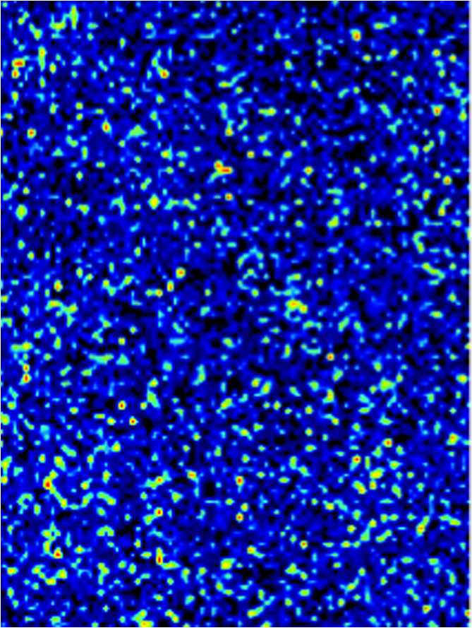
For LSCI data, our goal is to compare MSE values given by the sMSE algorithm with those given by the original MSE algorithm proposed by Costa et al.²¹^,²² For these two algorithms, the results obtained with different lengths for the shortest coarse-grained time series are studied.

2.3.

Measurement Procedure

The study was carried out in accordance with the Declaration of Helsinki. LSCI data were acquired on the dorsal face of the forearm of eight subjects (between 20 and 37 years old) without known disease. All the subjects provided written, informed consent prior to participation. LSCI is highly sensitive to movements. Therefore, the subjects had to be completely still during the acquisition. The participants were placed in a quiet room with controlled temperature and without any air movements,³⁵ see Fig. 1. LSCI data were acquired in arbitrary laser speckle perfusion units with a PeriCam PSI System (Perimed, Sweden) having a laser wavelength of 785 nm, a maximum output power of 70 mW, and an exposure time of 6 ms. The distance between the laser head and skin was set at 15.5 cm.³⁶ This gave images with a resolution of 0.44 mm (see an example in Fig. 2). In the imager used, the perfusion is computed as $Perfusion = k \times (1 / K - 1)$ , where $K$ is the contrast and $k$ is the signal gain factor. The signal gain factor is calibrated to ensure equal perfusion values for different instruments on a motility standard. The signal gain factor is instrument specific and may change after recalibration. LSCI images were acquired with a sampling frequency of 18 Hz on a computer. This sampling frequency has been chosen based on a previous work²⁷ and also to be able to capture the heart beats that could be the origin of the nonmonotonic evolution of MSE.²⁷ The recordings stopped when 23,000 images were recorded ( $\sim 22 \min$ of acquisition).

Fig. 1

Measurement setup (computer and head of the imager).

Fig. 2

Laser speckle contrast image of a zone on the forearm of a healthy subject.

2.4.

Implementation

For the implementation of the two algorithms on LSCI data (sMSE and original MSE algorithms), we randomly chose three pixels (noted hereafter as $P_{1}$ , $P_{2}$ , and $P_{3}$ ) in the first image of the time sequence of each subject.²⁷ Around each of these pixels, square ROIs were determined as (1) square of size $3 \times 3 {pixels}^{2}$ ( $1.74 {mm}^{2}$ ); (2) square of size $9 \times 9 {pixels}^{2}$ ( $15.68 {mm}^{2}$ ); (3) square of size $15 \times 15 {pixels}^{2}$ ( $43.56 {mm}^{2}$ ); (4) square of size $23 \times 23 {pixels}^{2}$ ( $102.41 {mm}^{2}$ ); (5) square of size $31 \times 31 {pixels}^{2}$ ( $186.05 {mm}^{2}$ ); (6) square of size $61 \times 61 {pixels}^{2}$ ( $720.39 {mm}^{2}$ ); (7) square of size $71 \times 71 {pixels}^{2}$ ( $975.93 {mm}^{2}$ ). For each ROI, the mean of the pixel values inside the ROI was computed and followed on each image of the sequence to obtain a time-evolution signal.³⁷ For each subject, we, therefore, had temporal signals from laser speckle contrast images that lasted at least 22 min (23,000 samples). The pixels $P_{1}$ , $P_{2}$ , and $P_{3}$ were also followed in the image sequence to obtain their time-evolution values. Then, the 192 ROIs (for each of the eight subjects, 3 pixels chosen and seven ROIs around each pixel + the pixels themselves) of eight different sizes (0.19 to $975.93 {mm}^{2}$ ) were processed with the two algorithms (sMSE and original MSE algorithms).

In our whole study, we implemented the two algorithms with standard parameter values $m = 2$ and $r = 0.15$ .²¹^,³⁴ Moreover, for all our data, a normalization has been performed before the application of the two algorithms (subtraction of the mean and division by the standard deviation). Finally, our work was conducted from scale factor $τ_{\min} = 1$ to scale factor $τ_{\max} = 23$ .

Costa et al. reported that the consistency of the original MSE algorithm is progressively lost when the number of samples in the time series decreases.²¹ The coarse-graining procedure generates time series with a decreasing number of data points, but the resulting time series is not a subset of the original sample sequence: the coarse-grained time series contains information about the entire original time series. Costa et al., therefore, mentioned that the error due to the decrease of coarse-grained time series length in the original MSE algorithm is lower than that resulting from selecting a subset of the original signal.²¹ One of our goals is to analyze MSE values given by the sMSE algorithm and by the original MSE algorithm when using different lengths for the shortest coarse-grained time series. Moreover, for all our computations, we studied MSE of LSCI data between scale factors $τ_{\min} = 1$ and $τ_{\max} = 23$ . Therefore, because $τ_{\max}$ is constant and because the shortest coarse-grained time series length varies, this amounts to working with original time series of different lengths. Several values for the shortest coarse-grained time series have been tested in our work: 1000, 500, 250, 200, 150, 100, and 50 samples. We, therefore, worked with signals of different lengths: 23,000 ( $23 \times 1000$ ) samples, 11,500 ( $23 \times 500$ ) samples, …, 1150 ( $23 \times 50$ ) samples.

Moreover, we first apply the two algorithms on two different kinds of synthetic signals with known expression for their multiscale entropy. The first kind of synthetic signal is a Gaussian white noise (mean: 0; variance: 1; uncorrelated noise). The second kind of synthetic signal is a $1 / f$ (long-range correlated) noise. Theoretical multiscale entropy values for white noise and $1 / f$ noise can be found in Ref. 21. For each of the two kinds of synthetic data, 24 signals have been generated. Here again, our study was performed for $τ_{\min} = 1$ to $τ_{\max} = 23$ .

2.5.

Statistical Analysis

Statistical analyses were performed using a Wilcoxon test.³⁸ We compared MSE values given by the original MSE algorithm when 1000 samples are chosen for the shortest coarse-grained time series with the ones given by the sMSE algorithm (using different lengths for the shortest coarse-grained time series) and with the ones given by the original MSE algorithm when $< 1000$ samples are chosen for the shortest coarse-grained time series. For each statistical analysis, a $p$ value $< 0.05$ was considered significant.

3. Results and Discussion

Figure 3 shows MSE values computed from the original MSE algorithm and from the sMSE algorithm for simulated Gaussian white noise. For the sMSE algorithm, the results obtained with several lengths for the shortest coarse-grained time series are shown: 1000, 500, and 50 samples. The statistical tests show that for all the lengths of the shortest coarse-grained time series tested in the sMSE algorithm (1000, 500, 250, 200, 150, 100, and 50 samples), the results obtained are not statistically different from those given by the original MSE algorithm when 1000 samples are chosen for the shortest coarse-grained time series.

Fig. 3

Multiscale entropy (MSE) values for white noise time series. Numerically estimated values obtained with the original MSE algorithm and with the short-time MSE (sMSE) algorithm are shown. For the original MSE algorithm, the shortest coarse-grained time series has 1000 samples. For the sMSE algorithm, results obtained with different lengths for the shortest coarse-grained time series are shown (1000, 500, and 50 samples). The line is the numerical evaluation of analytic MSE calculation (nits):²¹ $- \ln \int_{- \infty}^{+ \infty} (1 / 2) \sqrt{(τ / 2 π)} {\erf [(x + r) / \sqrt{2 / τ}] - \erf [(x - r) / \sqrt{2 / τ}]} \exp [(- x^{2} τ) / 2] d x$ , where $τ$ and $\erf ()$ refer to the scale factor and to the error function, respectively.

Figure 4 shows the MSE values computed from the original MSE algorithm and from the sMSE algorithm for simulated $1 / f$ noise. For the sMSE algorithm, the results obtained with several lengths for the shortest coarse-grained time series are shown: 1000, 500, and 50 samples. The statistical tests show that, when the length of the shortest coarse-grained time series in the sMSE algorithm is equal to 500 samples, the results obtained are not statistically different from those given by the original MSE algorithm when 1000 samples are chosen for the shortest coarse-grained time series. However, for the other lengths tested, the results are statistically different from the ones given by the original MSE algorithm when 1000 samples are chosen for the shortest coarse-grained time series (for all scales when 250, 200, 150, 100 or 50 samples are chosen).

Fig. 4

MSE values for $1 / f$ noise time series. Numerically estimated values obtained with the original MSE algorithm and with the sMSE algorithm are shown. For the original MSE algorithm, the shortest coarse-grained time series has 1000 samples. For the sMSE algorithm, results obtained with different lengths for the shortest coarse-grained time series are shown (1000, 500, and 50 samples). The line is the numerical evaluation of analytic MSE calculation:²¹ 1.8 nits for all scale factors $τ$ .

For LSCI data, our results show that, when the time evolution of LSCI single pixels is studied, the original MSE algorithm (with 1000 samples for the shortest coarse-grained time series) leads to a monotonic decreasing pattern, similar to the one of Gaussian white noise, see Fig. 5. However, when the mean of LSCI pixel values is computed in an ROI and followed with time, the original MSE algorithm (with 1000 samples for the shortest coarse-grained time series) leads to patterns where distinctive scales become visible for ROI large enough (see Figs. 5 Fig. 6 Fig. 7 to 8). These distinctive scales are found around $τ = 6$ and $τ = 17$ . These results are in accordance with a previous work where similar results have been reported.²⁷ Moreover, it has been suggested that origins of the distinctive scales could be dominated by the cardiac activity.³⁹ The sMSE algorithm (with 1000 samples for the shortest coarse-grained time series) leads to patterns that are similar to the ones obtained with the original MSE algorithm: a decreasing pattern with scales is observed when LSCI single pixels are studied with time and the emergence of distinctive scales for time evolution of ROI large enough (see Figs. 5 to 8). We find no statistical difference between the MSE values given by the two algorithms when 1000 samples are chosen for the shortest coarse-grained time series.

Fig. 5

MSE values (mean and standard deviations) obtained with 24 laser speckle contrast imaging (LSCI) time series computed from region of interest (ROI) sizes of $1 \times 1 {pixels}^{2}$ (a) and $3 \times 3 {pixels}^{2}$ (b) recorded in eight subjects without known disease. Numerically estimated MSE values obtained with the original MSE and with the sMSE algorithms using 1000 samples for the shortest coarse-grained time series are shown. Results given by the sMSE algorithm with the smallest length of the shortest coarse-grained time series, which leads to MSE values having no statistical difference from the ones given by the original MSE algorithm using different 1000 samples for the shortest coarse-grained time series, are also shown.

Fig. 6

MSE values (mean and standard deviations) obtained with 24 LSCI time series computed from ROI size of $9 \times 9 {pixels}^{2}$ (a) and $15 \times 15 {pixels}^{2}$ (b) recorded in eight subjects without known disease. Numerically estimated MSE values obtained with the original MSE and with the short-time MSE (sMSE) algorithms using 1000 samples for the shortest coarse-grained time series are shown. Results given by the sMSE algorithm with the smallest length of the shortest coarse-grained time series that leads to MSE values having no statistical difference with the ones given by the original MSE algorithm using different 1000 samples for the shortest coarse-grained time series are also shown.

Fig. 7

MSE values (mean and standard deviations) obtained with 24 LSCI time series computed from ROI sizes of $23 \times 23 {pixels}^{2}$ (a) and $31 \times 31 {pixels}^{2}$ (b) recorded in eight subjects without known disease. Numerically estimated MSE values obtained with the original MSE and with the sMSE algorithms using 1000 samples for the shortest coarse-grained time series are shown. Results given by the sMSE algorithm with the smallest length of the shortest coarse-grained time series, which leads to MSE values having no statistical difference from the ones given by the original MSE algorithm using different 1000 samples for the shortest coarse-grained time series, are also shown.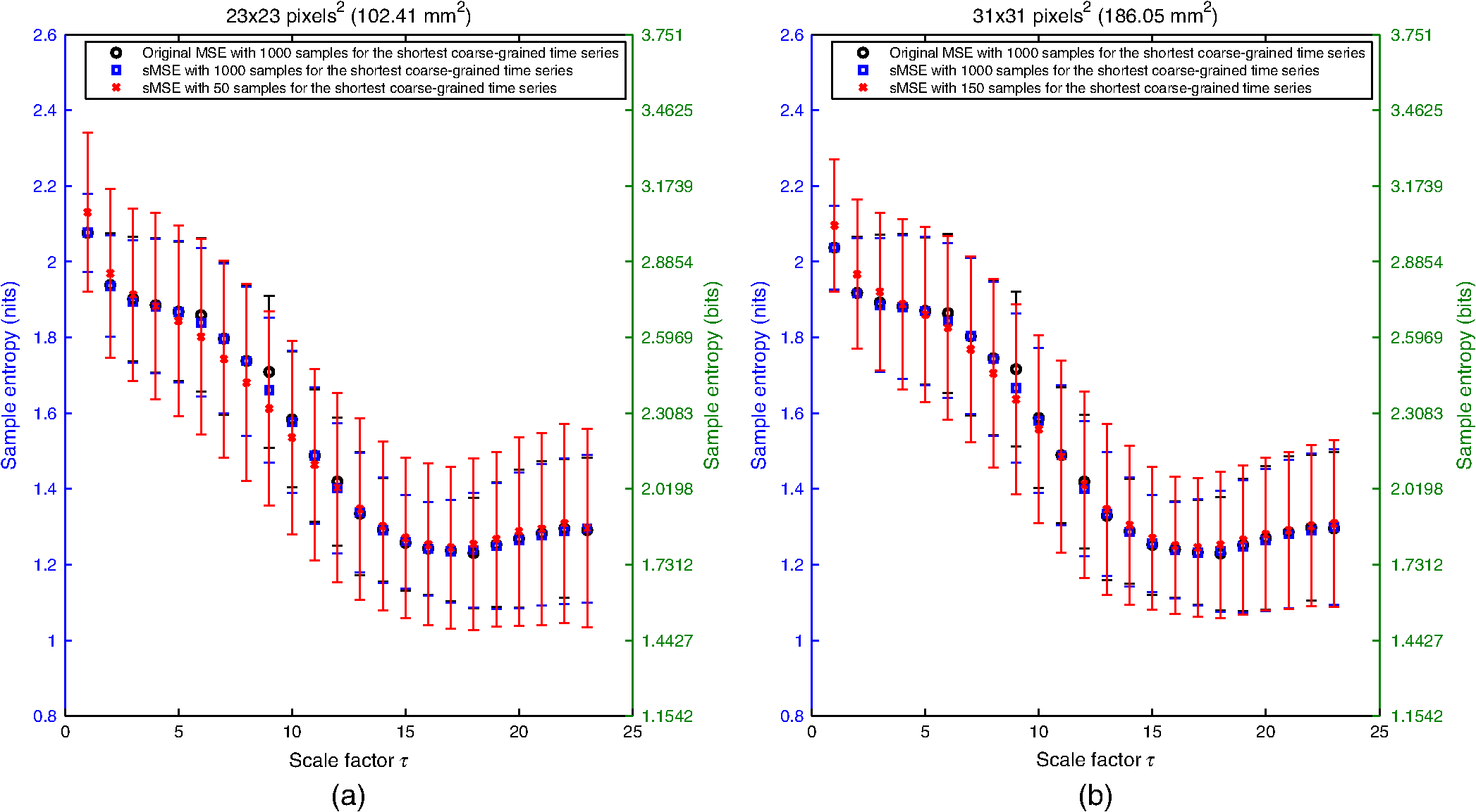

Fig. 8

MSE values (mean and standard deviations) obtained with 24 LSCI time series computed from ROI sizes of $61 \times 61 {pixels}^{2}$ (a) and $71 \times 71 {pixels}^{2}$ (b) recorded in eight subjects without known disease. Numerically estimated MSE values obtained with the original MSE and with the sMSE algorithms using 1000 samples for the shortest coarse-grained time series are shown. Results given by the sMSE algorithm with the smallest length of the shortest coarse-grained time series, which leads to MSE values having no statistical difference from the ones given by the original MSE algorithm using different 1000 samples for the shortest coarse-grained time series, are also shown.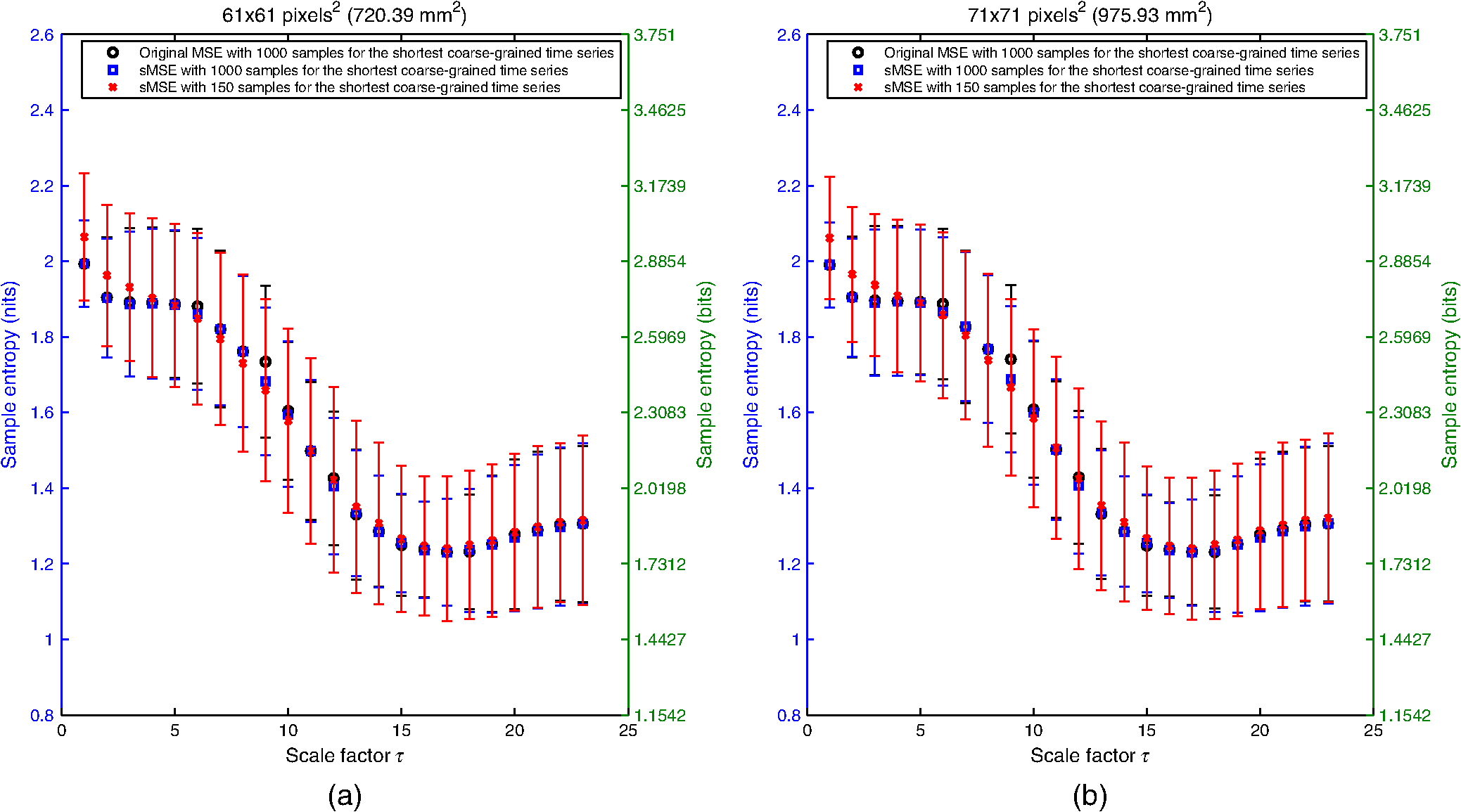

Table 1 shows the smallest lengths for the shortest coarse-grained time series, in the sMSE and original MSE algorithms, for which no statistical difference from the original MSE algorithm using 1000 samples for the shortest coarse-grained time series is found. The corresponding results are shown in Figs. 5 to 8. From Table 1, we observe that the length of the shortest coarse-grained time series in the sMSE algorithm that leads to results with no statistical difference from those given by the original MSE algorithm using 1000 samples for the shortest coarse-grained time series varies with the size of the LSCI ROI studied. The same conclusion can be drawn from the results obtained with the original MSE algorithm when different lengths are used for the shortest coarse-grained time series.

Table 1

Smallest length of the shortest coarse-grained time series—in the short-time multiscale entropy (sMSE) and in the original MSE algorithms—for which no statistical difference is found with the original MSE algorithm in which 1000 samples are chosen for the shortest coarse-grained time series. Results obtained for different regions of interest (ROI) sizes are shown. The results have been obtained testing different lengths for the shortest coarse-grained time series: 1000, 500, 250, 200, 150, 100, and 50 samples.

ROI size (pixels2)	Smallest length of the shortest coarse-grained time series in the sMSE algorithm for which no statistical difference is found with the original MSE algorithm in which 1000 samples are chosen for the shortest coarse-grained time series	Smallest length of the shortest coarse-grained time series in the original MSE algorithm for which no statistical difference is found with the original MSE algorithm in which 1000 samples are chosen for the shortest coarse-grained time series
$1 \times 1$	100 samples	100 samples
$3 \times 3$	200 samples	200 samples
$9 \times 9$	150 samples	50 samples
$15 \times 15$	50 samples	150 samples
$23 \times 23$	50 samples	50 samples
$31 \times 31$	150 samples	50 samples
$61 \times 61$	150 samples	50 samples
$71 \times 71$	150 samples	50 samples

Tables 2 and 3 show the lengths of the shortest coarse-grained time series, in the sMSE and original MSE algorithms, and associated scale factors, for which statistical differences from the original MSE algorithm in which 1000 samples are chosen for the shortest coarse-grained time series are found. From these tables, we observe that obtaining no statistical difference with a given length of the shortest coarse-grained time series (in the sMSE algorithm or original MSE algorithm) does not mean that no statistical difference is found for larger values of the shortest coarse-grained time series length. The analysis of these results deserve attention in future works.

Table 2

Lengths of the shortest coarse-grained time series—in the sMSE algorithm—and associated scale factors for which statistical differences are found from the original MSE algorithm in which 1000 samples are chosen for the shortest coarse-grained time series (left part of the table). The right part of the table shows the lengths of the shortest coarse-grained time series—in the original MSE algorithm—and the associated scale factors for which statistical differences are found from the original MSE algorithm in which 1000 samples are chosen for the shortest coarse-grained time series. Results obtained for different ROI sizes are shown.

ROI size (pixels2)	sMSE with coarse-grained time series shorter than 1000 samples		Original MSE with coarse-grained time series shorter than 1000 samples
ROI size (pixels2)	Size of the shortest coarse-grained time series	Scale factor	Size of the shortest coarse-grained time series	Scale factor
$1 \times 1$	50 samples	$τ = 1$ to 5	50 samples	$τ = 1$ to 5, 7 to 8, 13
$3 \times 3$	250 samples	$τ = 9$
$3 \times 3$	150 samples	$τ = 6$ , 9	150 samples	$τ = 6$ , 8, 14
$3 \times 3$	100 samples	$τ = 5$ to 19, 21 to 23	100 samples	$τ = 6$ to 12, 14, 17, 19, 20
$3 \times 3$	50 samples	$τ = 6$ , 9	50 samples	$τ = 14$ , 19
$9 \times 9$	250 samples	$τ = 1$
$9 \times 9$	100 samples	$τ = 2$	100 samples	$τ = 2$
$9 \times 9$	50 samples	$τ = 9$
$15 \times 15$	250 samples	$τ = 1$ , 2	250 samples	$τ = 1$
$15 \times 15$	200 samples	$τ = 1$ , 2	200 samples	$τ = 1$
$15 \times 15$	100 samples	$τ = 1$ , 2	100 samples	$τ = 1$ , 2
$15 \times 15$			50 samples	$τ = 2$

Table 3

Same as Table 2 but for other ROI sizes.

ROI size (pixels2)	sMSE with coarse-grained time series shorter than 1000 samples		Original MSE with coarse-grained time series shorter than 1000 samples
ROI size (pixels2)	Size of the shortest coarse-grained time series	Scale factor	Size of the shortest coarse-grained time series	Scale factor
$23 \times 23$	250 samples	$τ = 1$ , 2	250 samples	$τ = 1$ , 2
$23 \times 23$	200 samples	$τ = 1$
$23 \times 23$	100 samples	$τ = 1$ , 2	100 samples	$τ = 1$ , 2
$31 \times 31$	250 samples	$τ = 1$ , 2	250 samples	$τ = 1$ , 2
$31 \times 31$	200 samples	$τ = 1$	200 samples	$τ = 2$
$31 \times 31$	100 samples	$τ = 1$ , 2	100 samples	$τ = 2$
$31 \times 31$	50 samples	$τ = 9$
$61 \times 61$	250 samples	$τ = 1$ , 2	250 samples	$τ = 1$ , 2
$61 \times 61$	200 samples	$τ = 1$	200 samples	$τ = 1$ , 2
$61 \times 61$	100 samples	$τ = 1$	100 samples	$τ = 1$ , 2
$61 \times 61$	50 samples	$τ = 9$
$71 \times 71$	250 samples	$τ = 1$ , 2	250 samples	$τ = 1$ , 2
$71 \times 71$	200 samples	$τ = 1$	200 samples	$τ = 1$ , 2
$71 \times 71$	100 samples	$τ = 1$	100 samples	$τ = 1$
$71 \times 71$	50 samples	$τ = 9$

Our results lead to the conclusion that, for LSCI data, the sMSE algorithm is valid to compute MSE values. The length of the shortest coarse-grained time series that gives results that are not statistically different from those given by the original MSE algorithm when 1000 samples are chosen for the shortest coarse-grained time series depends on the ROI size studied (see Table 1). The same conclusion can be drawn for the original MSE algorithm when different lengths for the shortest coarse-grained time series are studied. Thus, for an ROI size of $3 \times 3 {pixels}^{2}$ , the optimal length for the shortest coarse-grained time series, both for the sMSE and original MSE algorithms, is 200 samples. This is five times lower than what was originally proposed in the original MSE algorithm. Thus, in order to study scale factors $τ$ from 1 to 23, we have to use $23 \times 200 = 4600$ samples instead of $23 \times 1000 = 23,000$ samples as initially proposed (use of 1000 samples for the shortest coarse-grained time series). For LSCI data recorded with a sampling frequency of 18 Hz, this means that 4.3 min are necessary instead of 21.3 min.

The main problem in using the MSE algorithm with LSCI data in a clinical setting was that long recordings were necessary in order to observe the patterns with distinctive scales. Because LSCI is very sensitive to movements, the subjects need to stay totally immobile. A total immobilization is difficult for periods as long as 21 min; our work overcomes this drawback because we show that the distinctive scales, which may be linked to central physiological activities, become accessible for periods of $\sim 4 \min$ . These findings make possible the design of studies including larger cohorts of healthy subjects and patients with a pathology where the microcirculation is affected (e.g., diabetes). It would now be interesting to determine if the MSE methodology would lead to relevant clinical data. For example, would the MSE pattern obtained from subjects with a microvascular disease be able to reveal systemic pathologies? Furthermore, for a patient with an acute myocardial infarction, could MSE pattern predict future cardiovascular events? Moreover, from previous papers where LSCI reproducibility has been studied,⁴⁰ we can hope that only one recording would be enough for such studies. Our work, therefore, serves as a basis for future studies of MSE analyses of LSCI data in clinical practice.

Other directions could also be studied in the future:

• In our study, we reduced the number of the original time series while keeping constant the highest scale factor studied ( $τ_{\max} = 23$ ). Therefore, the shortest coarse-grained time series was reduced with the reduction of the original time series length. For all our computations, we used the standard values for parameters $m$ and $r$ ( $m = 2$ and $r = 0.15$ ). In order to avoid spuriously high entropy values when reducing the time series length (high entropy values generated by the finding of none or very few matches in the computation), other work could be conducted in order to analyze the results obtained with less restrictive $r$ values.
• In our work, the lengths that have been tested for the shortest coarse-grained time series are 1000, 500, 250, 200, 150, 100, and 50 samples. The minimal length for the shortest coarse-grained time series was, therefore, set to 50 samples. No shorter length has been studied. The results that would arise from shorter lengths for the shortest coarse-grained time series remain to be studied. Other lengths (especially between 1000 and 500 samples) could also be tested. Moreover, further work could be conducted in order to analyze if the Bootstrap method of statistics could anticipate our results.
• Our analysis was conducted on MSE values; no entropy index (sum of sample entropy values over a predefined range of scales) has been computed, as proposed in other papers.²⁸^,³³ A study similar to the one presented herein could now be conducted when dealing with entropy indices.

References

1.

J. Allen and K. Howell, “Microvascular imaging: techniques and opportunities for clinical physiological measurements,” Physiol. Meas., 35 R91 –R141 (2014). http://dx.doi.org/10.1088/0967-3334/35/7/R91 PMEAE3 0967-3334 Google Scholar

2.

A. Humeau-Heurtier et al., “Relevance of laser Doppler and laser speckle techniques for assessing vascular function: state of the art and future trends,” IEEE Trans. Biomed. Eng., 60 659 –666 (2013). http://dx.doi.org/10.1109/TBME.2013.2243449 IEBEAX 0018-9294 Google Scholar

3.

J. Senarathna et al., “Laser speckle contrast imaging: theory, instrumentation and applications,” IEEE Rev. Biomed. Eng., 6 99 –110 (2013). http://dx.doi.org/10.1109/RBME.2013.2243140 1937-3333 Google Scholar

4.

D. Briers et al., “Laser speckle contrast imaging: theoretical and practical limitations,” J. Biomed. Opt., 18 066018 (2013). http://dx.doi.org/10.1117/1.JBO.18.6.066018 JBOPFO 1083-3668 Google Scholar

5.

D. A. Boas and A. K. Dunn, “Laser speckle contrast imaging in biomedical optics,” J. Biomed. Opt., 15 011109 (2010). http://dx.doi.org/10.1117/1.3285504 JBOPFO 1083-3668 Google Scholar

6.

A. K. Dunn et al., “Dynamic imaging of cerebral blood flow using laser speckle,” J. Cereb. Blood Flow Metab., 21 195 –201 (2001). http://dx.doi.org/10.1097/00004647-200103000-00002 JCBMDN 0271-678X Google Scholar

7.

J. Briers and S. Webster, “Laser speckle contrast analysis (LASCA): a nonscanning, full-field technique for monitoring capillary blood flow,” J. Biomed. Opt., 1 174 –179 (1996). http://dx.doi.org/10.1117/12.231359 JBOPFO 1083-3668 Google Scholar

8.

A. Fercher and J. Briers, “Flow visualization by means of single-exposure speckle photography,” Opt. Commun., 37 326 –330 (1981). http://dx.doi.org/10.1016/0030-4018(81)90428-4 OPCOB8 0030-4018 Google Scholar

9.

L. M. Richards et al., “Low-cost laser speckle contrast imaging of blood flow using a webcam,” Biomed. Opt. Express, 4 2269 –2283 (2013). http://dx.doi.org/10.1364/BOE.4.002269 BOEICL 2156-7085 Google Scholar

10.

J. C. Ramirez-San-Juan et al., “Spatial versus temporal laser speckle contrast analyses in the presence of static optical scatterers,” J. Biomed. Opt., 19 106009 (2014). http://dx.doi.org/10.1117/1.JBO.19.10.106009 JBOPFO 1083-3668 Google Scholar

11.

P. Miao et al., “Entropy analysis reveals a simple linear relation between laser speckle and blood flow,” Opt. Lett., 39 3907 –3910 (2014). http://dx.doi.org/10.1364/OL.39.003907 OPLEDP 0146-9592 Google Scholar

12.

C. Lal, A. Banerjee and N. U. Sujatha, “Role of contrast and fractality of laser speckle image in assessing flow velocity and scatterer concentration in phantom body fluids,” J. Biomed. Opt., 18 111419 (2013). http://dx.doi.org/10.1117/1.JBO.18.11.111419 JBOPFO 1083-3668 Google Scholar

13.

P. Miao et al., “Laser speckle contrast imaging of cerebral blood flow in freely moving animals,” J. Biomed. Opt., 16 090502 (2011). http://dx.doi.org/10.1117/1.3625231 JBOPFO 1083-3668 Google Scholar

14.

A. B. Parthasarathy et al., “Laser speckle contrast imaging of cerebral blood flow in humans during neurosurgery: a pilot clinical study,” J. Biomed. Opt., 15 066030 (2010). http://dx.doi.org/10.1117/1.3526368 JBOPFO 1083-3668 Google Scholar

15.

O. B. Thompson and M. K. Andrews, “Tissue perfusion measurements: multiple-exposure laser speckle analysis generates laser Doppler-like spectra,” J. Biomed. Opt., 15 027015 (2010). http://dx.doi.org/10.1117/1.3400721 JBOPFO 1083-3668 Google Scholar

16.

E. Figueiras et al., “Sample entropy of laser Doppler flowmetry signals increases in patients with systemic sclerosis,” Microvasc. Res., 82 152 –155 (2011). http://dx.doi.org/10.1016/j.mvr.2011.05.007 MIVRA6 0026-2862 Google Scholar

17.

W. Chen et al., “Measuring complexity using FuzzyEn, ApEn, and SampEn,” Med. Eng. Phys., 31 61 –68 (2009). http://dx.doi.org/10.1016/j.medengphy.2008.04.005 MEPHEO 1350-4533 Google Scholar

18.

A. Humeau et al., “Multifractality, sample entropy, and wavelet analyses for age-related changes in the peripheral cardiovascular system: preliminary results,” Med. Phys., 35 717 –723 (2008). http://dx.doi.org/10.1118/1.2831909 MPHYA6 0094-2405 Google Scholar

19.

D. Abasolo et al., “Entropy analysis of the EEG background activity in Alzheimer’s disease patients,” Physiol. Meas., 27 241 –253 (2006). http://dx.doi.org/10.1088/0967-3334/27/3/003 PMEAE3 0967-3334 Google Scholar

20.

D. E. Lake et al., “Sample entropy analysis of neonatal heart rate variability,” Am. J. Physiol. Regul. Integr. Comp. Physiol., 283 R789 –R797 (2002). 0363-6119 Google Scholar

21.

M. Costa, A. L. Goldberger and C. K. Peng, “Multiscale entropy analysis of biological signals,” Phys. Rev. E, 71 021906 (2005). http://dx.doi.org/10.1103/PhysRevE.71.021906 PLEEE8 1063-651X Google Scholar

22.

M. Costa, A. L. Goldberger and C. K. Peng, “Multiscale entropy analysis of complex physiologic time series,” Phys. Rev. Lett., 89 068102 (2002). http://dx.doi.org/10.1103/PhysRevLett.89.068102 PRLTAO 0031-9007 Google Scholar

23.

Z. Trunkvalterova et al., “Reduced short-term complexity of heart rate and blood pressure dynamics in patients with diabetes mellitus type 1: multiscale entropy analysis,” Physiol. Meas., 29 817 –828 (2008). http://dx.doi.org/10.1088/0967-3334/29/7/010 PMEAE3 0967-3334 Google Scholar

24.

J. Escudero et al., “Analysis of electroencephalograms in Alzheimer’s disease patients with multiscale entropy,” Physiol. Meas., 27 1091 –1106 (2006). http://dx.doi.org/10.1088/0967-3334/27/11/004 PMEAE3 0967-3334 Google Scholar

25.

H. Cao et al., “Toward quantitative fetal heart rate monitoring,” IEEE Trans. Biomed. Eng., 53 111 –118 (2006). http://dx.doi.org/10.1109/TBME.2005.859807 IEBEAX 0018-9294 Google Scholar

26.

U. Lee, S. Kim and S. H. Yi, “Event and time-scale characteristics of heart-rate dynamics,” Phys. Rev. E Stat. Nonlin. Soft Matter Phys., 71 061917 (2005). http://dx.doi.org/10.1103/PhysRevE.71.061917 PLEEE8 1539-3755 Google Scholar

27.

A. Humeau-Heurtier et al., “Multiscale entropy study of medical laser speckle contrast images,” IEEE Trans. Biomed. Eng., 60 872 –879 (2013). http://dx.doi.org/10.1109/TBME.2012.2208642 IEBEAX 0018-9294 Google Scholar

28.

M. D. Costa et al., “Dynamical glucometry: use of multiscale entropy analysis in diabetes,” Chaos, 24 033139 (2014). http://dx.doi.org/10.1063/1.4894537 CHAOEH 1054-1500 Google Scholar

29.

E. Guerreschi et al., “Complexity quantification of signals from the heart, the macrocirculation and the microcirculation through a multiscale entropy analysis,” Biomed. Signal Process. Control, 8 341 –345 (2013). http://dx.doi.org/10.1016/j.bspc.2013.04.001 1746-8094 Google Scholar

30.

Z. Turianikova et al., “The effect of orthostatic stress on multiscale entropy of heart rate and blood pressure,” Physiol. Meas., 32 1425 –1437 (2011). http://dx.doi.org/10.1088/0967-3334/32/9/006 PMEAE3 0967-3334 Google Scholar

31.

G. Mahe et al., “Cutaneous microvascular functional assessment during exercise: a novel approach using laser speckle contrast imaging,” Pflugers Arch., 465 (4), 451 –458 (2013). http://dx.doi.org/10.1007/s00424-012-1215-7 0031-6768 Google Scholar

32.

G. Mahé et al., “Laser speckle contrast imaging accurately measures blood flow over moving skin surfaces,” Microvasc. Res., 81 (2), 183 –188 (2011). http://dx.doi.org/10.1016/j.mvr.2010.11.013 MIVRA6 0026-2862 Google Scholar

33.

Y. C. Chang et al., “Application of a modified entropy computational method in assessing the complexity of pulse wave velocity signals in healthy and diabetic subjects,” Entropy, 16 4032 –4043 (2014). http://dx.doi.org/10.3390/e16074032 ENTRFG 1099-4300 Google Scholar

34.

J. S. Richman and J. R. Moorman, “Physiological time-series analysis using approximate entropy and sample entropy,” Am. J. Physiol. Heart Circ. Physiol., 278 H2039 –H2049 (2000). Google Scholar

35.

G. Mahe et al., “Air movements interfere with laser speckle contrast imaging recordings,” Lasers Med. Sci., 27 1073 –1076 (2012). http://dx.doi.org/10.1007/s10103-011-1015-x LMSCEZ 1435-604X Google Scholar

36.

G. Mahe et al., “Distance between laser head and skin does not influence skin blood flow values recorded by laser speckle imaging,” Microvasc. Res., 82 439 –442 (2011). http://dx.doi.org/10.1016/j.mvr.2011.06.014 MIVRA6 0026-2862 Google Scholar

37.

P. Rousseau et al., “Increasing the ‘region of interest’ and ‘time of interest,’ both reduce the variability of blood flow measurements using laser speckle contrast imaging,” Microvasc. Res., 82 88 –91 (2011). http://dx.doi.org/10.1016/j.mvr.2011.03.009 MIVRA6 0026-2862 Google Scholar

38.

J. D. Gibbons and S. Chakraborti, Nonparametric Statistical Inference, 5th ed.Chapman & Hall, CRC Press, Taylor & Francis Group, Boca Raton, FL (2011). Google Scholar

39.

A. Humeau et al., “Multiscale analysis of microvascular blood flow: a multiscale entropy study of laser Doppler flowmetry time series,” IEEE Trans. Biomed. Eng., 58 2970 –2973 (2011). http://dx.doi.org/10.1109/TBME.2011.2160865 IEBEAX 0018-9294 Google Scholar

40.

M. Roustit et al., “Excellent reproducibility of laser speckle contrast imaging to assess skin microvascular reactivity,” Microvasc. Res., 80 505 –511 (2010). http://dx.doi.org/10.1016/j.mvr.2010.05.012 MIVRA6 0026-2862 Google Scholar

Biography

Anne Humeau-Heurtier received her PhD degree in signal and image processing. She is currently a professor at the University of Angers, France. Her research interests are mainly focused on the processing of laser Doppler flowmetry data and laser speckle contrast images.

Guillaume Mahé is a medical doctor at the University Hospital of Rennes. He obtained his PhD in 2011 and is an assistant professor of vascular medicine at the University of Rennes, France. His main research activity is clinical research in the microcirculation field using laser and oximetry especially in patients with peripheral artery disease. Since his postdoctoral fellowship, he is a research collaborator at the Mayo Clinic (Rochester, MN, USA).

Pierre Abraham is a cardiologist and a professor of physiology at the University of Angers, France. His current research interest focuses on vascular physiology and exercise. Many of his recent papers are on the clinical use of microvascular devices.

Citation Download Citation

Anne Humeau-Heurtier, Guillaume Mahé, and Pierre Abraham "Modified multiscale sample entropy computation of laser speckle contrast images and comparison with the original multiscale entropy algorithm," Journal of Biomedical Optics 20(12), 121302 (28 July 2015). https://doi.org/10.1117/1.JBO.20.12.121302

Published: 28 July 2015

Access the abstract

JOURNAL ARTICLE
10 PAGES

DOWNLOAD PAPER SAVE TO MY LIBRARY

GET CITATION

CITATIONS

Cited by 4 scholarly publications.

Explore citations on Lens.org

RIGHTS & PERMISSIONS

Get copyright permission Get copyright permission on Copyright Marketplace

KEYWORDS

Laser speckle contrast imaging

Speckle

Statistical analysis

Signal processing

Cardiovascular system

Data acquisition

Biomedical optics

1.

Introduction