Offset-sparsity decomposition for automated enhancement of color microscopic image of stained specimen in histopathology

Ivica Kopriva; Marijana Popović Hadžija; Mirko Hadžija; Gorana Aralica

doi:10.1117/1.JBO.20.7.076012

28 July 2015 Offset-sparsity decomposition for automated enhancement of color microscopic image of stained specimen in histopathology

Ivica Kopriva, Marijana Popović Hadžija, Mirko Hadžija, Gorana Aralica

Author Affiliations +

Journal of Biomedical Optics, Vol. 20, Issue 7, 076012 (July 2015). https://doi.org/10.1117/1.JBO.20.7.076012

Abstract

We propose an offset-sparsity decomposition method for the enhancement of a color microscopic image of a stained specimen. The method decomposes vectorized spectral images into offset terms and sparse terms. A sparse term represents an enhanced image, and an offset term represents a “shadow.” The related optimization problem is solved by computational improvement of the accelerated proximal gradient method used initially to solve the related rank-sparsity decomposition problem. Removal of an image-adapted color offset yields an enhanced image with improved colorimetric differences among the histological structures. This is verified by a no-reference colorfulness measure estimated from 35 specimens of the human liver, 1 specimen of the mouse liver stained with hematoxylin and eosin, 6 specimens of the mouse liver stained with Sudan III, and 3 specimens of the human liver stained with the anti-CD34 monoclonal antibody. The colorimetric difference improves on average by 43.86% with a 99% confidence interval (CI) of [35.35%, 51.62%]. Furthermore, according to the mean opinion score, estimated on the basis of the evaluations of five pathologists, images enhanced by the proposed method exhibit an average quality improvement of 16.60% with a 99% CI of [10.46%, 22.73%].

1. Introduction

Visualization of different tissue structures in a histological specimen and the corresponding microscopic analysis undertaken by pathologists is still a basic clinical workflow required for an assessment of specimens and for diagnosing a disease. That is, pathologists look for visual cues to distinguish between healthy and diseased tissues. In this regard, various stains and tags are attached to biological tissues to improve the colorimetric difference between the tissue components (histological structures), thereby improving their visibility.¹^,² For example, it is known that in hematoxylin–eosin (H&E)-stained slides, color information is essential to discriminate between healthy and diseased tissues.³^,⁴ However, because of the variations in the tissue preparation processes such as collection, preservation, sectioning, staining, and illumination, the tissue color and texture can vary considerably between specimens. These nonbiological experimental variations are also known as batch effects.⁵^,⁶ For example, variation in the spectral signature of the stained tissue creates noise at image acquisition; this noise is also known as biochemical noise.³^,⁷ These variations can change the quantitative morphological image features, and this makes it difficult to reach an accurate diagnosis,⁵ e.g., in the field of digital pathology, i.e., computerized image analysis⁸ that has entered an era of computer-assisted diagnosis and treatment of medical conditions based on an analysis of medical images.²^,⁹^–¹² For example, accurate segmentation of the images of H&E-stained slides is very challenging because of the weak (fuzzy) boundaries between histological structures.¹¹ The variations discussed above create additional difficulties in this regard. Further, the diagnosis of hepatocellular carcinoma is based on the extraction/segmentation of the trabecula, a specific structure of liver cells, whose extraction from an H&E-stained specimen of the liver tissue could sometimes be difficult.¹³ This difficulty is attributed to the fact that the extraction of this structure is highly affected by the variation of color and/or texture of the tissue.¹³ Variability in the received colors also creates difficulties in an automated diagnosis of gastric cancer performed on H&E-stained gastric tissue sections.¹⁴ Thus, as emphasized in some studies,¹⁵^,¹⁶ standardization of the H&E staining process is one of the key prerequisites of computer-aided systems to produce accurate clinical data for use by anatomical pathology diagnosis assisting systems. Furthermore, as shown in a recent study,¹⁷ pathology experts are sensitive to color variations. Further, specimen-dependent variation in the color and/or texture of a tissue causes disagreement in diagnosis between pathologists; this disagreement can lead to a difference of up to 20% in the diagnoses.¹⁸

The abovementioned problems related to the variations in the quality of the staining process were the motivation for the development of an automated image enhancement method, particularly for enhancing the colorimetric difference between the histological structures present in the images of a stained specimen. Further, in order to be practically relevant, we require such a method to be truly unsupervised, i.e., a method that does not require any prior information from the user and is completely data driven. Such a method would also need to demonstrate the validity and robustness of performance on images of different tissues stained, possibly, by various stains. Therefore, we propose an automated image enhancement method that is based on the decomposition of an unfolded color image of a stained specimen into a sum of the approximately constant offset matrix and the sparse matrix, which denotes an improved image with an enhanced colorimetric difference between histological structures. The proposed method can be seen as a special (degenerative) case of the rank-sparsity decomposition (RSD) that decomposes a matrix into a sum of low-rank and sparse matrices.¹⁹^,²⁰ The method proposed herein decomposes vectorized spectral images into a sum of an approximately constant offset vector and a sparse vector. We have named the proposed method the offset-sparsity decomposition (OSD) method. In this method, the offset term corresponds to the $ℓ_{2}$ -norm-based regularization and the sparse term corresponds to the $ℓ_{1}$ -norm-based regularization in an optimization problem related to the minimization of the difference between the vectorized spectral images and the model. Further, because the proposed method is similar to RSD, the accelerated proximal gradient method²¹^–²⁴ used for solving the RSD problem can be used for OSD as well, since for a vector, the nuclear norm equals the $ℓ_{2}$ -norm, and the related optimization problem in the OSD case is simpler than in the RSD case. That is, the thresholded singular value decomposition (SVD) required by nuclear norm (low-rank) regularization in the RSD problem is trivial to compute for $ℓ_{2}$ -norm regularization in the OSD problem. The most often suggested application of RSD is related to the detection of rare events from surveillance videos.¹⁹^,²⁵ Therefore, the background is contained in a low-rank matrix and the foreground (which accounts for rare events) is held in a sparse matrix. Another often suggested application of RSD is related to the removal of shadows and specularities from face images,¹⁹ thus increasing the accuracy of face recognition. Herein, to the best of our knowledge, we propose for the first time, an application of novel OSD to color microscopic images of a stained specimen in order to enhance the perception of details (histological structures) and to improve the colorimetric difference between the histological structures contained in the image. From this perspective, the image adaptive offset removal by the OSD method is, to some extent, analogous to the removal of shadows from face images by means of RSD.¹⁹ In particular, we propose the decomposition of an original color image by executing OSD on vectorized grayscale intensity images that correspond to red, green, and blue (RGB) colors. We call this method the OSD_rgb algorithm. The OSD-based approach to image enhancement differs from the $ℓ_{1}$ -norm-based sparsity-regularized denoising, implemented by soft thresholding (ST),²⁶^–²⁸ in the following important aspects: sparsity-regularized denoising is based on an additive data model consisting of noiseless data and noise. The proposed OSD method models data as an additive superposition of the offset term, noiseless data, and noise. The proposed method, together with ST and the $L^{1}$ -retinex algorithm,²⁹^–³¹ is illustrated in Fig. 1 using an enhancement of an image of an H&E-stained specimen of the human liver [Fig. 1(a)]. The color offset term is shown in Fig. 1(b), whereas Fig. 1(c) shows an enhanced image that is captured by the “sparse” term and is of actual interest. Figure 1(d) shows the image enhanced by denoising that is based on ST in the wavelet domain, whereas Fig. 1(e) shows the image enhanced by the $L^{1}$ -retinex algorithm.²⁹

Fig. 1

Flowchart of the OSD approach to the enhancement of a color microscopic image of the stained specimen. Information on image quality metrics such as mean opinion score (MOS), colorfulness, sharpness, and contrast can be found in Sec. 2.3. (a) Hematoxylin and eosin (H&E) stained specimen of human liver with metastasis from colon cancer: $MOS = 4.2$ , $colorfulness = 0.446$ , $sharpness = 9.38$ , $contrast = 1.77$ . (b) Color offset term obtained by OSD_rgb algorithm. (c) Image enhanced with OSD_rgb algorithm: $MOS = 5$ , $colorfulness = 0.619$ , $sharpness = 9.42$ , $contrast = 1.57$ . (d) Image enhanced with the double-density dual-tree discrete wavelet transform soft thresholding Stein’s unbiased risk estimator (DDDTDWT-ST-SURE) algorithm: $MOS = 3.8$ , $colorfulness = 0.443$ , $sharpness = 7.08$ , $contrast = 1.87$ . (e) Image enhanced with the $L^{1}$ -retinex algorithm: $MOS = 2.8$ , $colorfulness = 0.305$ , $sharpness = 13.75$ , and $contrast = 1.05$ .

The assumption upon which the proposed OSD_rgb approach to image enhancement relies is that after the removal of the image adaptive color offset, the enhanced image will be sparser than the original image. Thus, such an image will contain more information than the original image; i.e., its entropy will be lower than the entropy of the original image. This is attributed to the fact that the sparser the stochastic process is, the more is its probability density function concentrated around the mode(s). Consequently, the Fisher information, which is a measure of the degree of disorder of a system, will increase (the degree of disorder will be lower; i.e., the signal will be more predictable).³² Thus, details are expected to be better perceived in the enhanced image than in the original image. It is, therefore, expected that the proposed method will reduce the artifacts caused by the previously discussed variations and standardize the quality of the acquired histopathological images. Thus, the OSD_rgb method can be used as a preprocessing method to produce images with an improved colorimetric difference between the histological structures, and this should help a pathologist to better perceive visual cues and assess diagnoses. The OSD_rgb method can possibly be used in computerized image analysis systems, such as the classification and/or segmentation methods discussed in Ref. 3, for a computer-assisted diagnosis complementary to a human pathologist. However, the ability of the OSD_rgb method to increase the classification rate of a computerized image analysis system has not been demonstrated in the current study. In particular, the collection of samples with annotations (diagnoses) and the selection of features necessary to build predictive models are critical steps that require significant effort. In this study, by using a no-reference-image measure of colorimetric information,³³ we have demonstrated that the OSD_rgb method yields an image with an improved colorimetric difference between the histological structures. Further, the performance of the OSD method is compared with that of the $L^{1}$ -retinex algorithm²⁹^–³¹ and that of the ST of coefficients in a domain obtained using a double-density dual-tree discrete wavelet transform (DDDTDWT).³⁴ DDDTDWT has improved directional selectivity and can be used for implementing complex and directional wavelet transforms in multiple dimensions. This makes it suitable for image denoising/enhancement problems. The MATLAB code for two-dimensional (2-D) DDDTDWT has been downloaded from Ref. 35. Denoising has been performed by using ST coefficients at the first resolution level. Further, the threshold has been estimated adaptively by using the MATLAB function thselect with an option for Stein’s unbiased risk estimator (SURE).³⁶^,³⁷ We call this approach to denoising/enhancement the DDDTDWT-SURE-ST method. The $L^{1}$ -retinex algorithm performs image enhancement on the value $V$ component of the image in the hue-saturation-value (HSV) color space.³⁸ The MATLAB code that implements the $L^{1}$ -retinex algorithm, as an alternative to the more general nonlocal retinex method,²⁹^,³⁰ is available in Ref. 39.

The rest of this paper is organized as follows: the details of the OSD_rgb method are presented in Sec. 2. This is followed by an experimental comparative performance analysis in Sec. 3 and the discussion in Sec. 4. The summary and conclusions are presented in Sec. 5.

2. Materials and Methods

2.1.

Notations and Related Works

Within this paper, we use the following notation: an underlined upper-case bold letter, e.g., $\underset{̲}{X} \in R_{0 +}^{I_{1} \times I_{2} \times 3}$ , denotes a three-dimensional (3-D) RGB image tensor consisting of three spectral images corresponding with the red, green, and blue colors, where each image measures $I_{1} \times I_{2}$ pixels. An upper-case bold letter, e.g., $X$ , denotes a matrix; a lower-case bold letter, e.g., $x$ , denotes a vector; and an italicized lower-case letter, e.g., $x$ , denotes a scalar. The random variable $e$ that follows the Gaussian distribution with zero mean and variance $σ^{2}$ is denoted as $e \sim N (0, σ^{2})$ . The standard model of the observed image assumed by many image denoising methods is as follows:²⁶^–²⁸^,⁴⁰

Eq. (1)

b_{n} = s_{n} + e_{n} n \in {1,2, 3},

where

b_{n} \in R_{0 +}^{1 \times I_{1} I_{2}}

stands for the intensity of the observed vectorized spectral image at a particular color channel,

s_{n} \in R_{0 +}^{1 \times I_{1} I_{2}}

stands for a noiseless but unknown image that is to be estimated, and

e_{n} \sim N (0, σ_{n}^{2} I)

stands for the additive white Gaussian noise (AWGN). Under the AWGN assumption, an optimal estimate of

s_{n}

is obtained by solving the log-likelihood problem that is regularized by the addition of a wavelet-domain

ℓ_{1}

-penalty (a.k.a. sparseness constraint):

Eq. (2)

\min_{c_{s_{n}}} {{‖ c_{b_{n}} - c_{s_{n}} ‖}_{2}^{2} + λ {‖ c_{s_{n}} ‖}_{1}},

where

c_{b_{n}}

and

c_{s_{n}}

denote the vectors of coefficients in a wavelet basis. The exact solution of Eq. (2) is then obtained by ST as follows:²⁶^,²⁷^,⁴¹

Eq. (3)

c_{s_{n}} = S_{λ / 2} (c_{b_{n}}) = \max (c_{b_{n}} - λ / 2,0),

such that the max operator is applied entry-wise. An estimate of

s_{n}

is obtained through the inverse wavelet transform

D

:

{\hat{s}}_{n} = {Dc}_{s_{n}}

. While an optimal value of the regularization constant

λ

in Eqs. (2) and (3) is proportional to

σ_{n}^{2}

, SURE enables its estimate from

c_{b_{n}}

. In Eq. (2), we assume that

c_{s_{n}}

is sparse, but this depends on how well the chosen basis represents the data (image). From this perspective, 2-D DDDTDWT,³⁴ because of its directivity, represents a good choice for the transformation domain. In addition to fixed transforms, we can consider the learned ones.⁴²^,⁴³

The retinex methodology assumes that an observed image is a multiplication of the illumination and reflection intensity terms, whereas the reflection term represents an enhanced image. Therefore, the retinex method is applied to the value $V$ channel in the HSV color space as follows:

Eq. (4)

v (i_{1}, i_{2}) = i (i_{1}, i_{2}) r (i_{1}, i_{2}),

where

(i_{1}, i_{2})

denotes the pixel location;

i

denotes the illumination (shadow) term; and

r

denotes the reflection term that is of actual interest. By taking logarithm

v_{\log} = \log (v)

, etc., we can obtain an additive impact of the illumination as follows:³¹

Eq. (5)

v_{\log} (i_{1}, i_{2}) = i_{\log} (i_{1}, i_{2}) + r_{\log} (i_{1}, i_{2}),

where

r_{\log}

is then estimated as a solution of the optimization problem; see also Sec. 6 [Sec. 6.1.3 and Eq. (6.13)] in Ref. 29:

Eq. (6)

{\hat{r}}_{\log} = \min_{r_{\log}} {{‖ \nabla_{w} r_{\log} - \nabla_{w},_{f} i_{\log} ‖}_{1} + α {‖ r_{\log} ‖}_{2} + β {‖ r_{\log} - i_{\log} ‖}_{2}},

where

\nabla_{w} r_{\log}

stands for the nonlocal gradient of

r_{\log}

, see also Definition 3.7 in Ref. 29, and

\nabla_{w},_{f} i_{\log}

stands for the nonlocal filtered gradient of

i_{\log}

, see also Definition 3.12 in Ref. 29. As proposed in Ref. 29, in an example related to shadow removal from an image of a natural scene, we select

α = β = 0.5

and a hard thresholding filter

f

with a threshold set to 0.015. Then,

r

is estimated as

\hat{r} = imadjust {\exp ({\hat{r}}_{\log}) / \max [\exp ({\hat{r}}_{\log})]}

,³¹^,³⁹ where imadjust represents a MATLAB image enhancement command. A retinex-enhanced color image is then obtained by transforming the enhanced value channel component

\hat{r}

image from the HSV back to the RGB color space.

2.2.

Offset-Sparsity Decomposition

In contrast to Eqs. (1), (4), and (5), we propose the following model for the intensity of the observed spectral images of a color microscopic image:

Eq. (7)

b_{n} = s_{n} + a_{n} + e_{n} n \in {1,2, 3},

where the term

s_{n}

denotes the noiseless but unknown image, while the term

a_{n}

represents an offset that, in the spirit of Ref. 19, will model shadows present in the image due to various batch effects.⁵ The proposed OSD method aims to estimate

a_{n}

and

s_{n}

by using only

b_{n}

. After matricization,

{a_{n} \in R_{0 +}^{1 \times I_{1} I_{2}} \to A_{n} \in R_{0 +}^{I_{1} \times I_{2}}}_{n = 1}^{3}

and tensorisation

{\underset{̲}{A} (:, :, n) = A_{n}}_{n = 1}^{3}

,

\underset{̲}{A}

represents the image-adapted color offset.

\underset{̲}{S} \in R_{0 +}^{I_{1} \times I_{2} \times 3}

, formed analogously from

{s_{n} \in R_{0 +}^{1 \times I_{1} I_{2}}}_{n = 1}^{3}

, represents an enhanced color microscopic image with, in comparison with the original image

\underset{̲}{B}

, an improved colorimetric difference between the histological structures present in the specimen. Under the AWGN assumption, the optimal estimates of

a_{n}

and

s_{n}

are obtained by solving the log-likelihood problem regularized by the addition of

ℓ_{2}

- and

ℓ_{1}

-penalties as follows:

Eq. (8)

({\hat{a}}_{n}, {\hat{s}}_{n}) = \min_{(a_{n}, s_{n})} {\frac{1}{2} {‖ b_{n} - a_{n} - s_{n} ‖}_{2}^{2} + μ {‖ a_{n} ‖}_{2} + μ λ {‖ s_{n} ‖}_{1}} .

Equation (8) can be considered a special case of the RSD problem:¹⁹^–²¹

Eq. (9)

(\hat{A}, \hat{S}) = \min_{(A, S)} {\frac{1}{2} {‖ B - A - S ‖}_{F}^{2} + μ {‖ A ‖}_{*} + μ λ {‖ S ‖}_{1}},

where

B = A + S

with the dimensions

I_{1} \times I_{2}

. Therefore,

{‖ A ‖}_{*}

denotes the nuclear norm of a matrix (sum of its singular values) that is used in Eq. (9) as a convex relaxation of the nondeterministic polynomial-hard rank minimization problem.²³ Equation (9) is also known as robust principal component analysis, in Ref. 19, which aims to recover a low-rank matrix

A

in the presence of the corruption

S

with a sparse structure and possibly large values. Equation (9) admits a unique solution with the value of the regularization parameter set to

λ = 1 / \sqrt{\max (I_{1}, I_{2})}

.¹⁹^,²⁰ The fast proximal gradient (FPG) optimization method is used for solving Eq. (9).²¹ To this end, let us denote

X = (A, S)

,

g (X) = {‖ A ‖}_{*} + λ {‖ S ‖}_{1}

,

f (X) = \frac{1}{2} {‖ B - A - S ‖}_{F}^{2}

. Then, Eq. (9) can be written as follows:

Eq. (10)

\hat{X} = \min_{X} F (X) ≐ f (X) + μ g (X) .

A computationally efficient solution of Eq. (10) is obtained using proximal gradient algorithms, as shown in Refs. 21–24, that minimize the sequence of the quadratic approximations to $F (X)$ , denoted as $Q (X, Y)$ , formed at specially chosen points $Y$ for Lipschitz constant $L > 0$ :

Eq. (11)

Q (X, Y) ≐ f (Y) + 〈 \nabla f (Y), X - Y 〉 + \frac{L}{2} {‖ X - Y ‖}_{F}^{2} + μ g (X) .

By defining

h (Y) ≐ Y - \frac{1}{L} \nabla f (Y)

, we can reduce the minimization of Eq. (11) to the following:²¹^–²⁴

Eq. (12)

\underset{X}{\arg \min} Q (X, Y) = \underset{X}{\arg \min} {μ g (X) + \frac{L}{2} {‖ X - h (Y) ‖}_{F}^{2}} .

By setting $Y_{k} = X_{k} + \frac{t_{k - 1} - 1}{t_{k}} (X_{k} - X_{k - 1})$ , where $k$ denotes the iteration index for a sequence, the $t_{k} = (1 + \sqrt{1 + 4 t_{k - 1}^{2}}) / 2$ convergence of Eq. (12) is made quadratic.²²^,⁴⁴ When $g (X) = λ {‖ S ‖}_{1}$ , Eq. (12) has a closed-form solution $S_{k + 1} = S_{\frac{λ μ}{L}} (h (Y_{k}^{S}))$ . When $g (X) = {‖ A ‖}_{*}$ , Eq. (12) has a closed-form solution $A_{k + 1} = U S_{μ / L} (Σ) V^{T}$ , where $U Σ V^{T}$ stands for the SVD of $h (Y_{k}^{A})$ . Rank minimization, implied by the minimization of a nuclear norm, is not suitable for solving Eq. (8), which is a special case of Eq. (9), when matrices $B$ , $A$ , and $S$ are reduced to vectors. However, since for a vector ${‖ a_{n} ‖}_{2} = {‖ a_{n} ‖}_{*}$ , the nuclear norm minimization from Eq. (9) is reduced to the $ℓ_{2}$ -norm minimization in Eq. (8), and Eq. (8) for $g (x) = {‖ a_{n} ‖}_{2}$ has, like Eq. (9), a closed-form solution $a_{n (k + 1)} = u S_{μ / L} (σ) v^{T}$ , where $u σ v^{T}$ is the SVD of $h (y_{k}^{a_{n}})$ . However, in the case of a vector, the SVD is trivial to compute. For a row vector $h (y_{k}^{a_{n}})$ , $u = 1$ , $σ = {‖ h (y_{k}^{a_{n}}) ‖}_{2}$ , and $v^{T} = h (y_{k}^{a_{n}}) / {‖ h (y_{k}^{a_{n}}) ‖}_{2}$ . Thus, the closed-form solution of a vector equivalent to Eq. (12) related to the minimization of ${‖ a_{n} ‖}_{2}$ is computationally very efficient:

Eq. (13)

a_{n (k + 1)} = S_{μ / L} ({‖ h (y_{k}^{a_{n}}) ‖}_{2}) h (y_{k}^{a_{n}}) / {‖ h (y_{k}^{a_{n}}) ‖}_{2} .

The closed-form solution of a vector equivalent to Eq. (12) for $g (x) = λ {‖ s_{n} ‖}_{1}$ is a standard ST solution of the $ℓ_{1}$ -norm regularized least square problem:²⁶^,²⁷

Eq. (14)

s_{n (k + 1)} = S_{\frac{λ μ}{L}} [h (y_{k}^{s_{n}})] .

Thus, we can formulate a computationally efficient solution of the OSD problem [Eq. (8)] by using the FPG method, used in Ref. 21 to solve the RSD problem [Eq. (9)]. To this end, Algorithm 2 in Ref. 21 is adopted to solve Eq. (8) such that the SVD computation step is trivial to compute; see Eq. (13). As in the case of the RSD problem defined in Eq. (9), the sparsity-related regularization constant $λ$ in the OSD problem [Eq. (8)] is set to $λ = 1 / \sqrt{\max (1, I_{1} \times I_{2})} = 1 / \sqrt{I_{1} \times I_{2}}$ . We summarize the OSD FPG method in Algorithm 1.

Algorithm 1

The OSD FPG algorithm.

Input: observed vectorized spectral image $b_{n} \in R_{0 +}^{1 \times I_{1} I_{2}}$ , sparsity regularization constant $λ$ , regularization constant $μ$ , Lipschitz constant $L$ .

1.

a_{n (0)} = 0

;

a_{n (- 1)} = 0

;

s_{n (0)} = 0

;

s_{n (- 1)} = 0

;

t_{0} = t_{- 1} = 1

.

2. while not converge do

3.

y_{k}^{a_{n}} \leftarrow a_{n (k)} + \frac{t_{k - 1} - 1}{t_{k}} [a_{n (k)} - a_{n (k - 1)}], y_{k}^{s_{n}} \leftarrow s_{n (k)} + \frac{t_{k - 1} - 1}{t_{k}} [s_{n (k)} - s_{n (k - 1)}]

4.

h (y_{k}^{a_{n}}) \leftarrow y_{k}^{a_{n}} - \frac{1}{L} (y_{k}^{a_{n}} + y_{k}^{s_{n}} - b_{n})

.

5.

a_{n (k + 1)} = S_{μ / L} ({‖ h (y_{k}^{a_{n}}) ‖}_{2}) h (y_{k}^{a_{n}}) / {‖ h (y_{k}^{a_{n}}) ‖}_{2}

6.

h (y_{k}^{s_{n}}) \leftarrow y_{k}^{s_{n}} - \frac{1}{L} (y_{k}^{a_{n}} + y_{k}^{s_{n}} - b_{n})

7.

s_{n (k + 1)} = S_{\frac{λ μ}{L}} (h (y_{k}^{s_{n}}))

8.

t_{k + 1} \leftarrow \frac{1 + \sqrt{4 t_{k}^{2} + 1}}{2}

9.

k \leftarrow k + 1

10. end while

Output: $a_{n} \leftarrow a_{n (k + 1)}, s_{n} \leftarrow s_{n (k + 1)}$ .

To avoid the color artifacts, the enhancement of the color images is preferably executed in the CIE $L^{*} a^{*} b^{*}$ color space instead of the RGB color space. In the case of the OSD_rgb approach to color image enhancement, which operates independently on the color channels in RGB color space, color artifacts are avoided because of the following reason: even though the optimization problem implied by Eq. (8) is independently solved for each channel, the data fidelity terms, ${2^{- 1} {‖ b_{n} - a_{n} - s_{n} ‖}_{2}^{2}}_{n = 1}^{3}$ , prevent enhanced spectral images ${s_{n}}_{n = 1}^{3}$ to deviate significantly from the experimental spectral image ${b_{n}}_{n = 1}^{3}$ . Because of the same reason, the intensity offsets ${a_{n}}_{n = 1}^{3}$ that are independently extracted in each spectral channel, when merged together, yield the image adapted color offset term. In addition to Fig. 1, this can be seen in Figs. 2 and 3 in Sec. 3. We summarize the OSD_rgb algorithm in Algorithm 2.

Fig. 2

Images of the H&E-stained specimen of (a) and (b) human fatty liver; (c) hepatocellular carcinoma. (d)–(f): Images enhanced with OSD_rgb algorithm corresponding to stained images (a)–(c), respectively. (g)–(i): Color offset images obtained by OSD_rgb algorithm corresponding to stained images (a)–(c), respectively. (j)–(l): Images enhanced with $L^{1}$ -retinex algorithm corresponding to stained images (a)–(c), respectively. (m)–(o): Shadow images obtained by $L^{1}$ -retinex algorithm corresponding to stained images (a)–(c), respectively. (p)–(r): Images enhanced with DDDTDWT-ST-SURE algorithm corresponding to stained images (a)–(c), respectively.

Fig. 3

(a) Image of the H&E-stained specimen of human liver with hepatocellular carcinoma. (b) Image of anti-CD34-stained specimen of human fatty liver. (c) Image of Sudan III-stained specimen of mouse fatty liver. (d)–(f): Images enhanced with OSD_rgb algorithm corresponding to stained images (a)–(c), respectively. (g)–(i): Color offset images obtained by OSD_rgb algorithm corresponding to stained images (a)–(c), respectively. (j)–(l): Images enhanced with $L^{1}$ -retinex algorithm corresponding to stained images (a)–(c), respectively. (m)–(o): Shadow images obtained by $L^{1}$ -retinex algorithm corresponding to stained images (a)–(c), respectively. (p)–(r): Images enhanced with DDDTDWT-ST-SURE algorithm corresponding to stained images (a)–(c), respectively.

Algorithm 2

The OSD_rgb algorithm for the enhancement of a color microscopic image of the stained specimen.

Input: $B \in R_{0 +}^{3 \times I_{1} I_{2}}$ unfolded color image of the stained specimen with vectorized grayscale images ${b_{n} \in R_{0 +}^{1 \times I_{1} I_{2}}}_{n = 1}^{3}$ measuring $I_{1} \times I_{2}$ pixels. Sparsity regularization constant in Eq. (8): $λ = 1 / \sqrt{I_{1} \times I_{2}}$ , regularization constant in Eq. (8): $μ = 1 0^{- 3}$ , threshold constant in Eqs. (13) and (14): $L = 2$ .

for $n = 1 ∶ 3$

(a_{n}, s_{n}) = Algorithm 1 (b_{n}, λ, μ, L)

.

end for

Set: $A = [\begin{matrix} a_{1} \\ a_{2} \\ a_{3} \end{matrix}]$ , $S = [\begin{matrix} s_{1} \\ s_{2} \\ s_{3} \end{matrix}]$ .

Output: $S \in R_{0 +}^{3 \times I_{1} I_{2}}$ unfolded enhanced color image of the stained specimen. $A \in R^{3 \times I_{1} I_{2}}$ unfolded image with the color offset term. The enhanced color image is obtained by tensorizing $S$ : $\underset{̲}{S} \in R_{0 +}^{I_{1} \times I_{2} \times 3}$ .

2.3.

Performance Measure

To quantify the performance of image enhancement algorithms, appropriate measures have to be defined. In the case of a color microscopic image of the stained specimen, the primary concern is the improvement of the colorimetric difference between the histological structures.² To this end, we estimate the colorfulness attribute, as discussed in Ref. 33, directly from the image. It measures the amount of chrominance information that humans perceive. This attribute plays an important role in the quality of the color image of the stained specimen.²^,¹⁷ The colorfulness measure is defined as follows:³³

Eq. (15)

colorfulness = 0.02 \times \log (\frac{σ_{α}^{2}}{{| μ_{α} |}^{0.2}}) \times \log (\frac{σ_{β}^{2}}{{| μ_{β} |}^{0.2}}),

where

α = red - green

color images;

β = 0.5 \times (red + green) - blue

color images; and

σ_{α}^{2}

,

σ_{β}^{2}

,

μ_{α}

, and

μ_{β}

represent the variance and mean along the

α

and

β

opponent color axes, respectively. In addition to the colorfulness measure, which is objective, we have asked five independent pathology experts to evaluate the images of routinely stained specimens as well as the enhanced images. The images were graded on the scale from 1 to 5. Grade 5 refers to quality that yields the best perception of details in histological structures. This enabled us to obtain the mean opinion score (MOS) quality measure for images of stained specimens as well as for enhanced images. Even though they are not of primary concern, we have also estimated the sharpness and contrast measures, as discussed in Ref. 33, from the original and enhanced images. Sharpness is the attribute related to the preservation of fine details (edges) in a color image. As described in Ref. 33, the Sobel edge detector is applied to each RGB color component. Then binary edge maps are multiplied with the original values to obtain three grayscale edge maps. The grayscale edge maps are used as enhancement measure (EME) by measuring the Weber contrast in a small window (

3 \times 3

pixels in the case of this study):

{EME}_{sharpness} = \frac{2}{k_{1} k_{2}} \sum_{i = 1}^{k_{1}} \sum_{j = 1}^{k_{2}} \log (\frac{I_{\max, i, j}}{I_{\min, i, j}}),

where

k_{1}

and

k_{2}

denote the number of blocks across image dimensions, and

I_{\max, i, j}

and

I_{\min, i, j}

represent the maximal and minimal intensity value in each window, respectively. The sharpness measure for the color image is then obtained as follows:³³

Eq. (16)

Sharpness = \sum_{c = 1}^{3} λ_{c} {EME}_{sharpness} ({grayedge}_{c}),

where the weighting coefficients for the red, green, and blue components are as follows:

λ_{1} = 0.299

,

λ_{2} = 0.587

, and

λ_{3} = 0.114

. Contrast is defined as the ratio of the maximum and the minimum intensity of the entire image.³³ Therefore, for a color image, it is calculated on the luminance component

L^{*}

in the CIE

L^{*} a^{*} b^{*}

color space.

3. Experiments and Results

The OSD_rgb image enhancement method has been comparatively evaluated on 35 specimens of the human liver, 1 specimen of the mouse liver stained with H&E, 6 specimens of the mouse liver stained with Sudan III, and 3 specimens of the human liver stained with the anti-CD34 monoclonal antibody. The detailed diagnostic information is given in Table 1. Descriptions of the experimental setup are given below.

Table 1

Information on specimens used for evaluating the performance of the OSD_rgb image enhancement method.

Stain	Human liver: diagnosis and number of specimens	Mouse liver: diagnosis and number of specimens
H&E Total: 36	Fatty liver: 14; hepatocellular carcinoma: 8; metastasis of colon cancer: 12; metastasis of pancreatic adenocarcinoma: 1	Fatty liver: 1
Sudan III Total: 6		Fatty liver: 6
Anti-CD34 antibody Total: 3	Fatty liver: 3

3.1.

Ethics Statements

This study was approved by the Bioethics Committee of the Ruđer Bošković Institute (BP-2290/2-2012) and the Clinical Hospital Dubrava Ethics Committee (October 10, 2013).

3.2.

Samples of Human Liver Tissue

All tissue samples of the human liver ( $N = 38$ ) were obtained from the repository of Department of Pathology and Cytology, Clinical Hospital Dubrava, Zagreb. After surgical liver resection or a liver needle biopsy, the tissue was routinely processed (fixed in 4% formalin for 24 to 48 h, embedded in paraffin blocks, cut on a microtome into 4 to $5 - μ m$ -thick tissue sections, and stained with H&E). The pathologists then diagnostically evaluated the samples as follows: fatty liver, hepatocellular carcinoma, liver metastasis of colon cancer, or pancreatic adenocarcinoma (see Table 1). The sections were deparaffinized and rehydrated according to the standard protocols.⁴⁵ Antigen retrieval was performed by microwaving the sections at 750 W in a 10-mM citrate buffer (pH 6.0) for $2 \times 5 \min$ , followed by the acquisition of a color microscopic image or immunohistochemical staining.

3.3.

Immunochemical Staining

Staining of the human liver section with the CD34 antigen is used for discriminating blood vessels from other similar structures within the liver tissue. After antigen retrieval, endogenous tissue peroxides were quenched by immersion in 0.3% $H_{2} O_{2}$ in phosphate buffered saline (PBS) for 30 min at room temperature, followed with three buffer washes. Dako EnVision/DAB kit (Dako, Denmark) was used for blocking no-specific antibody binding. The primary anti-CD34 antibody (Clone QBEnd10, Dako, Denmark) was applied in dilution 1:50 in PBS and incubated for 1 h in a humidified chamber. Then the sections were washed two times in PBS and incubated with a secondary antibody (peroxidase-labeled polymer conjugated to goat anti-mouse immunoglobulins in a Tris–HCl buffer) for 1 h. The activity of the peroxidase molecules was visualized with 3,3-diaminobenzidine (Dako) followed by counterstaining with hematoxylin. The sections were analyzed under a light microscope (Olympus BX51 with a DP50 camera, Japan; magnification: $200 \times$ or $400 \times$ ), and the images were taken at almost the same position as the images of the H&E-stained sections.

3.4.

Animal Studies

Eight-week-old male CBA mice were purchased from animal facilities at Ruđer Bošković Institute. Animals were maintained in standard conditions on chow diet or on a high-fat diet containing 58% fat, 16.4% proteins, and 25.6% carbohydrates (Mucedolla, Italy) for a period of 20 weeks. At the end of the experiment, the animals were euthanized by an overdose of Ketamidor 10% (Richter Pharma AG, Wels, Austria). The liver was immediately removed, fixed in Bouin’s solution (picric acid, saturated aqueous solution—75 ml; formalin, 40% aqueous solution—25 ml; acetic acid, glacial—5 ml) for at least 4 h, washed in PBS, and preserved by immersion in 30% (w/v) sucrose (Kemika, Zagreb, Croatia) in PBS overnight. Small pieces of the liver tissue were immersed in an OCT compound (Sakura, Netherland), frozen in isopentane, cooled by liquid nitrogen, and cryosectioned at $8 μ m$ in a freezing cryostat (Leica, Austria). After incubation in a series of tap and distilled water and ethanol, the frozen sections were incubated in a Sudan III working solution (0.1% Sudan III solution in 70% alcohol) for 30 min and then washed in distilled water. The sections were then counterstained with hematoxylin and viewed under a light microscope.

3.5.

Color Microscopic Image Acquisition and Processing

The RGB color images of the slides were acquired at room temperature in the mounting medium (10% glycerol in PBS) under the fluorescence microscope Olympus BX51 with a DP50 camera having a numerical aperture of the objective lens of 1/120, a magnification of $200 \times$ or $400 \times$ , and Viewfinder Lite 1.0 image acquisition software. Each acquired color microscopic image was stored as a 3-D tensor $\underset{̲}{X} \in R_{0 +}^{I_{1} \times I_{2} \times 3}$ consisting of three grayscale images (corresponding to red, green, and blue colors) measuring $I_{1} \times I_{2}$ pixels ( $I_{1} = 2074$ , $I_{2} = 2776$ ). Prior to processing, the images were downsampled by a factor of two by using the MATLAB imresize command. Thus, the size of the processed images was $1037 \times 1388$ pixels. For the purpose of the image analysis, the image tensor $\underset{̲}{X}$ was unfolded into a matrix $X \in R_{0 +}^{3 \times I_{1} I_{2}}$ . That is, the grayscale images were vectorized and stored as row vectors measuring $1 \times I_{1} I_{2}$ elements. The images were analyzed with software written in the MATLAB® (the MathWorks Inc., Natick, MA) script language. The OSD_rgb algorithm took 32.12 s, the $L^{1}$ -retinex algorithm took 5254 s, and the 2-D DDDTDWT-SURE-ST algorithm took 7.36 s for the processing.

3.6.

Comparative Results

Here, we present the results of the comparative performance analysis between the OSD_rgb algorithm, the $L^{1}$ -retinex algorithm,²⁹ and the 2-D DDDTDWT-SURE-ST algorithm.³⁴^,³⁶ Because 2-D DDDWT requires the number of pixels along each dimension to be a power of 2, a block measuring $1024 \times 1024$ pixels had to be extracted from the original image measuring $1037 \times 1388$ pixels. Comparative results obtained by the three methods are shown in Fig. 2 for three images stained using H&E, and in Fig. 3 for three images stained using H&E, anti-CD34 monoclonal antibody, and Sudan III, respectively. In addition to the enhanced images, we show the offset images estimated by the OSD_rgb method and the shadow images estimated by the $L^{1}$ -retinex method. The values of the estimated quality measures, calculated relative to the corresponding values estimated from the original images, are reported in Tables 2 and 3. Images enhanced by the OSD_rgb method had the highest colorfulness measure, which is crucial for increasing the colorimetric difference between histological structures. The $L^{1}$ -retinex method yielded very sharp images, but with extremely low colorfulness measure. The 2-D DDDTDWT-SURE-ST algorithm yielded enhanced (denoised) images with the highest contrast and an increased colorfulness measure with respect to the original images. Finally, according to the relative MOS measure, the OSD_rgb-enhanced images enabled the best perception of details; this is in agreement with the highest value of the colorfulness attribute for the OSD_rgb-enhanced images.

Table 2

Relative values, in percentage, of quality measures for images shown in Fig. 2. For each image, the best value for each measure is in bold.

	OSD_rgb			L1-retinex			DDDTDWT-SURE-ST
	(d)	(e)	(f)	(j)	(k)	(l)	(p)	(q)	(r)
Colorful	38.6	50.24	62.92	$- 40.57$	$- 49.53$	$- 30.55$	11.62	10.61	$- 3.66$
MOS	10	13.63	13.63	$- 20.00$	$- 50.00$	$- 36.36$	$- 15.00$	$- 13.63$	$- 4.54$
Sharpness	0.14	0.25	0.38	68.44	71.18	28.34	$- 21.76$	$- 21.11$	$- 23.60$
Contrast	$- 9.84$	$- 10.33$	$- 12.43$	$- 65.28$	$- 39.13$	$- 49.11$	0.52	3.8	5.92

Table 3

Relative values, in percentage, of quality measures for images shown in Fig. 3. For each image, the best value for each measure is in bold.

	OSD_rgb			L1-Retinex			DDDTDWT-SURE-ST
	(d)	(e)	(f)	(j)	(k)	(l)	(p)	(q)	(r)
Colorful	39.51	107.47	62.47	$- 37.32$	$- 39.86$	19.88	5.12	38.43	6.9
MOS	25.00	15.00	56.25	$- 55.00$	$- 70.00$	$- 6.25$	0.00	15.00	0.00
Sharpness	1.84	0.82	0.31	16.94	83.42	80.16	$- 21.55$	$- 12.48$	$- 29.84$
Contrast	$- 14.1$	$- 8.29$	$- 8.42$	$- 57.05$	$- 37.07$	$- 39.11$	10.9	0	2.97

In Fig. 4, we present the relative values of colorfulness, MOS, sharpness, and contrast measures estimated from 45 images enhanced by the OSD_rgb, $L^{1}$ -retinex, and 2-D DDDTWT-SURE-ST algorithms as well as from 45 stained images described in Table 1. In addition to images shown in Figs. 1 2–3, the original and the OSD_rgb-enhanced images are shown in Figs. 5 Fig. 6–7. Table 4 contains the mean values and the 99% confidence interval (CI), estimated from the relative values by using the MATLAB command ttest. The OSD_rgb method yields a statistically significant improvement of colorfulness (mean value: 43.86% and 99% CI: [41.59%, 59.13%]) and MOS (mean value: 16.60% and 99% CI: [10.46%, 22.73%]). It yields a statistically insignificant improvement of sharpness and yields a small but statistically significant decrease in contrast. The $L^{1}$ -retinex algorithm yields a statistically significant improvement of sharpness and a large, statistically significant decrease in colorfulness, contrast, and MOS. The 2-D DDDTDWT-SURE-ST yields a small but statistically significant improvement of colorfulness, a small but statistically significant decrease in MOS, and a statistically significant decrease in sharpness. Overall, the OSD_rgb method is the only one that significantly improves the colorfulness attribute, and this is crucial for increasing the colorimetric difference between the histological structures present in the image of the stained specimen. This is indirectly confirmed by the highest value of the relative MOS measure for the OSD_rgb method.

Table 4

Mean values and 99% confidence interval (CI) of the estimated relative image quality measures. The best values are in bold.

	Colorfulness		MOS		Sharpness		Contrast
	Mean (%)	99% CI (%)	Mean (%)	99% CI (%)	Mean (%)	99% CI (%)	Mean (%)	99% CI (%)
OSD_rgb	43.86	[35.35, 51.62]	16.60	[10.46, 22.73]	1.45	$[- 1.97, 4.86]$	$- 10.78$	$[- 13.16, - 8.4]$
$L^{1}$ -Retinex	$- 26.31$	$[- 33.67, - 18.95]$	$- 37.40$	$[- 47.27, - 27.54]$	50.36	[41.59, 59.13]	$- 45.73$	$[- 50.21, - 41.25]$
DDDTDWT-SURE-ST	6.84	[2.51, 11.17]	$- 3.67$	$[- 6.62, - 0.71]$	$- 21.56$	$[- 23.23, - 19.89]$	5.16	[2.61, 7.71]

Fig. 4

Relative values of (a) colorfulness measure, (b) MOS measure, (c) sharpness measure, and (d) contrast measure. Forty-five images were enhanced by algorithms according to the following legend: squares: OSD_rgb algorithm, circles: $L^{1}$ -retinex algorithm, and diamonds: 2-D DDDTDWT-SURE-ST algorithm.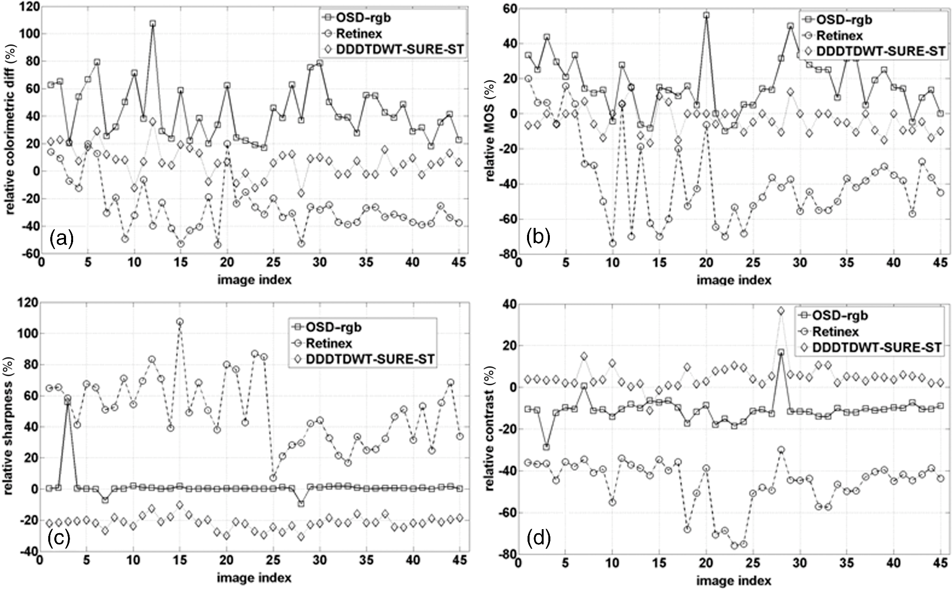

Fig. 5

(a)–(d): H&E-stained specimen of human fatty liver. (e)–(h): OSD_rgb-enhanced images corresponding to images of stained specimens (a)–(d), respectively. Specimens of human fatty liver: (i) and (j): anti-CD34-stained; (k) H&E-stained. (l) H&E-stained specimen of human liver with metastasis of colon cancer. (m)–(p): Images enhanced with OSD_rgb algorithm corresponding to images of stained specimens (i)–(l), respectively. (q) H&E-stained specimen of human fatty liver. (r) H&E-stained specimen of human liver with metastasis of gastric cancer. (s) and (t) H&E-stained human liver with hepatocellular carcinoma. (u)–(x): Images enhanced with OSD_rgb algorithm corresponding to images of stained specimens (q)–(t), respectively.

Fig. 6

(a)–(d): H&E-stained specimen of human fatty liver. (e)–(h): OSD_rgb-enhanced images corresponding to images of stained specimens (a)–(d), respectively. (i)–(l): Sudan III-stained specimens of mouse fatty liver. (m)–(p) OSD_rgb-enhanced images corresponding to images of stained specimens (i)–(l), respectively. (q) H&E-stained specimen of human fatty liver. (r) H&E-stained specimen of mouse fatty liver. (s) H&E-stained human liver with metastasis of colon cancer. (t) Sudan III-stained specimen of mouse fatty liver. (u)–(x): Images enhanced with OSD_rgb algorithm corresponding to images of stained specimens (q)–(t), respectively.

Fig. 7

(a)–(c): H&E-stained specimens of human liver with hepatocellular carcinoma. (d) H&E-stained specimen of human liver with metastasis of colon cancer. (e)–(h): OSD_rgb-enhanced images corresponding to images of stained specimens (a)–(d), respectively. (i)–(l): H&E-stained specimen of human liver with metastasis of colon cancer. (m)–(p): OSD_rgb-enhanced images corresponding to images of stained specimens (i)–(l), respectively. (q)–(t): H&E-stained specimen of human liver with metastasis of colon cancer. (u)–(x): Images enhanced with OSD_rgb algorithm corresponding to images of stained specimens (q)–(t), respectively.

3.7.

Description of Prognostic Information

The increased prognostic value of the OSD_rgb enhanced images is justified by a better perception of the details of the histological structures present in the specimen. To this end, visibility of the histological details in the OSD_rgb enhanced images is compared with that in the microscopic images of the liver specimens stained with H&E dye in Fig. 3(a), monoclonal antibody to CD34 antigen in Fig. 3(b), and Sudan III dye in Fig. 3(c). Blue nuclei, pink cytoplasm, pale brown cell membrane, gray extracellular space, and pink collagen fibers are more clearly visible in the OSD_rgb-enhanced image in Fig. 3(d) than in the image of the H&E-stained section in Fig. 3(a). Likewise, the location of the monoclonal antibody binding to the specific antigen on the endothelial cells, which is marked by brown, is easier to determine on the OSD_rgb-enhanced image in Fig. 3(e) than in the anti-CD34-stained image shown in Fig. 3(b). Moreover, it is known that the slides produced by a frozen section are of a lower quality than those produced by formalin fixed paraffin embedded tissue processing. Therefore, the staining of the cryosection yields a fuzzy image such as that of the cryosection of the mouse fatty liver stained with Sudan III, as shown in Fig. 3(c). However, in the OSD_rgb-enhanced image shown in Fig. 3(f), it is possible to see vacuoles with triglycerides (orange), nucleus (blue), and extracellular space (pink).

4. Discussion

Tissue samples obtained by different methods can vary in shape, size, and/or quality. Because of the used method and variations in the conditions of histological processing (such as fixation, dehydration, antigen retrieval, and sectioning), tissue color and texture can also vary. To address the abovementioned issues, the OSD_rgb method for an automated (unsupervised) enhancement of the color images of a stained specimen is proposed and demonstrated herein. It performs additive decomposition of the vectorized color images of an RGB color image of a stained specimen into a color offset term and a “sparse” term that stands for the enhanced image, as shown in Fig. 1 and Eq. (7). The proposed method is virtually free of user intervention and yields images of the stained specimen with an improved colorimetric difference between the histological structures as measured by the colorfulness attribute. This, according to the MOS, contributes decisively to the quality improvement of the OSD_rgb-enhanced images when compared with the original images as well as with images enhanced with the $L^{1}$ -retinex and the 2-D DDDTDWT-SURE-ST methods. This is expected to lead to a better recognition of the histological structures present in the specimen. This, in turn, is required for a quantitative assessment of histology and a further diagnosis of the disease. The performance of the OSD_rgb method is demonstrated on 36 images of the H&E-stained specimens of the human and mouse livers, 6 images of the Sudan III-stained specimens of the mouse liver, and 3 images of the anti-CD34-stained specimens of the human liver with a variety of diagnoses, as shown in Figs. 2, 3, and 5 Fig. 6–7. As shown in Fig. 4 and Table 4, the OSD_rgb method yields a statistically significant and consistent improvement of the colorfulness attribute as well as MOS. This is important for the standardization of the staining processes that are still frequently used in diagnostic pathology. It is conjectured that the OSD_rgb method can be used for enhancing images stored in various databases available for educational and learning purposes. It could also be applied in a routine clinical workflow and for an accurate pathology assessment of other tissues and/or organs. Therefore, the applicability of the OSD_rgb method to other types of staining, e.g., reticulin by silver impregnation should be tested.⁴⁶ Furthermore, it is conjectured that the proposed OSD method can be useful in enhancing images with a large dynamic range that, consequently, causes a loss of important details such as edges. In such a case, the OSD-based removal of the offset term is expected to yield more accurate edge detection results.

5. Conclusion

We have developed a new method for the automated enhancement of a color microscopic image of a stained specimen in histopathology and have named it the OSD_rgb method. This method was demonstrated on images of specimens stained with H&E, Sudan III, and anti-CD34 monoclonal antibody. The OSD_rgb method, compared to the original images of stained specimens, improved the colorimetric difference by an average of 43.86% with 99% CI of [35.35%, 51.62%]. On the basis of MOS, we concluded that the OSD_rgb-enhanced images, compared with the original images of the stained specimens, improved quality by an average of 16.60% with 99% CI of [10.46%, 22.73%]. Therefore, we conclude that the OSD_rgb method can complement pathologists in looking for visual cues and in assessing a diagnosis.

Acknowledgments

This work has been supported through Grant 9.01/232 “Nonlinear Component Analysis with Applications in Chemometrics and Pathology” funded by the Croatian Science Foundation. We would like to express our sincere gratitude to Arijana Pačić and Petar Šenjug for grading images of stained specimens and images produced by enhancement algorithms.

References

1.

J. M. Crawford and A. D. Burt, “Anatomy, pathophysiology and basic mechanism of disease,” Pathology of the Liver, 1 –77 6th ed.Elsevier, Churchill Livingstone (2011). Google Scholar

2.

P. A. Bautista and Y. Yagi, “Digital simulation of staining in histopathology multispectral images: enhancement and linear transformation of spectral transmittance,” J. Biomed. Opt., 17 (5), 056013 (2012). http://dx.doi.org/10.1117/1.JBO.17.5.056013 JBOPFO 1083-3668 Google Scholar

3.

M. Gavrilovic et al., “Blind color decomposition of histological images,” IEEE Trans. Med. Imaging, 32 (6), 983 –994 (2013). http://dx.doi.org/10.1109/TMI.2013.2239655 ITMID4 0278-0062 Google Scholar

4.

O. Sertel et al., “Histopathological image analysis using model-based intermediate representations and color texture: follicular lymphoma grading,” J. Signal Process. Syst., 55 (1–3), 169 –183 (2009). http://dx.doi.org/10.1007/s11265-008-0201-y Google Scholar

5.

S. Kothari et al., “Removing batch effects from histopathological images for enhanced cancer diagnosis,” IEEE J. Biomed. Health Inf., 18 (3), 765 –772 (2014). http://dx.doi.org/10.1109/JBHI.2013.2276766 Google Scholar

6.

J. H. Phan et al., “Multiscale integration of -omic, imaging, and clinical data in biomedical informatics,” IEEE Rev. Biomed. Eng., 5 74 –87 (2012). http://dx.doi.org/10.1109/RBME.2012.2212427 Google Scholar

7.

K. R. Castleman et al., “Classification accuracy in multiple color fluorescence imaging microscopy,” Cytometry, 41 (2), 139 –147 (2000). http://dx.doi.org/10.1002/1097-0320(20001001)41:2<139::AID-CYTO9>3.0.CO;2-N CYTODQ 0196-4763 Google Scholar

8.

A. J. Mendez et al., “Computer-aided diagnosis: automatic detection of malignant masses in digitized mammograms,” Med. Phys., 25 957 –964 (1998). http://dx.doi.org/10.1118/1.598274 MPHYA6 0094-2405 Google Scholar

9.

Y. Yagi, “Color standardization and optimization in whole slide imaging,” Diagn. Pathol., 6 (Suppl. 1), S15 (2011). http://dx.doi.org/10.4103/2153-3539.126153 DMPAES 1052-9551 Google Scholar

10.

U. Srinivas et al., “Simultaneous sparsity model for histopathological image representation and classification,” IEEE Trans. Med. Imaging, 33 (5), 1163 –1179 (2014). http://dx.doi.org/10.1109/TMI.2014.2306173 ITMID4 0278-0062 Google Scholar

11.

M. T. McCann et al., “Images as occlusions of textures: a framework for segmentation,” IEEE Trans. Image Process., 23 (5), 2033 –2046 (2014). http://dx.doi.org/10.1109/TIP.2014.2307475 IIPRE4 1057-7149 Google Scholar

12.

M. N. Gurcan et al., “Histopathological image analysis: a review,” IEEE Rev. Biomed. Eng., 2 147 –171 (2009). http://dx.doi.org/10.1109/RBME.2009.2034865 Google Scholar

13.

M. Ishikawa et al., “Automatic segmentation of hepatocellular structure from HE-stained liver tissue,” Proc. SPIE, 8676 867611 (2013). http://dx.doi.org/10.1117/12.2006669 PSISDG 0277-786X Google Scholar

14.

E. Cosatto et al., “Automated gastric cancer diagnosis on H&E stained sections: training a classifier on a large scale with multiple instance machine learning,” Proc. SPIE, 8676 867605 (2013). http://dx.doi.org/10.1117/12.2007047 PSISDG 0277-786X Google Scholar

15.

M. Ogura et al., “The e-pathologist cancer diagnosis assistance system for gastric biopsy tissues,” Anal. Cell. Pathol., 34 184 –185 (2011). ACPAER 0921-8912 Google Scholar

16.

A. Basavanhally and A. Madabhushi, “EM-based segmentation-driven color standardization of digitized histopathology,” Proc. SPIE, 8676 86760G (2013). http://dx.doi.org/10.1117/12.2007173 PSISDG 0277-786X Google Scholar

17.

L. Platiša et al., “Psycho-visual evaluation of image quality attributes in digital pathology slides viewed on a medical color LCD display,” Proc. SPIE, 8676 86760J (2013). http://dx.doi.org/10.1117/12.2006991 PSISDG 0277-786X Google Scholar

18.

J. J. Erasmus et al., “Interobserver and intraobserver variability in measurement of non small cell carcinoma lung lesions: implications for assessment of tumor response,” J. Clin. Oncol., 21 2574 –2582 (2003). http://dx.doi.org/10.1200/JCO.2003.01.144 JCONDN 0732-183X Google Scholar

19.

E. J. Candès et al., “Robust principal component analysis?,” J. ACM, 58 11 (2011). http://dx.doi.org/10.1145/1970392.1970395 Google Scholar

20.

V. Chandrasekaran et al., “Rank-sparsity incoherence for matrix decomposition,” SIAM J. Optim., 21 572 –596 (2011). http://dx.doi.org/10.1137/090761793 Google Scholar

21.

Z. Lin et al., Fast convex optimization algorithms for exact recovery of a corrupted low-rank matrix (2009). Google Scholar

22.

A. Beck and M. Teboulle, “A fast iterative shrinkage-thresholding algorithm for linear inverse problems,” SIAM J. Imaging Sci., 2 (1), 183 –202 (2009). http://dx.doi.org/10.1137/080716542 Google Scholar

23.

K. C. Toh and S. Yun, “An accelerated proximal gradient algorithm for nuclear norm regularized least square problems,” Pac. J. Opt., 6 (3), 615 –640 (2010). Google Scholar

24.

M. Fukushima and H. Mine, “A generalized proximal point algorithm for certain non-convex minimization problems,” Int. J. Syst. Sci., 12 (8), 989 –1000 (1981). http://dx.doi.org/10.1080/00207728108963798 Google Scholar

25.

N. S. Aybat, D. Goldfarb and S. Ma, “Efficient algorithms for robust and stable principal component pursuit problems,” Comput. Optim. Appl., 58 (1), 1 –29 (2014). http://dx.doi.org/10.1007/s10589-013-9613-0 CPPPEF 0926-6003 Google Scholar

26.

D. Donoho, “De-noising by soft-thresholding,” IEEE Trans. Inf. Theory, 41 (3), 613 –627 (1995). http://dx.doi.org/10.1109/18.382009 IETTAW 0018-9448 Google Scholar

27.

I. Daubechies, M. Defrise and C. De Mol, “An iterative thresholding algorithm for linear inverse problems with a sparisty constraint,” Commun. Pure Appl. Math., 57 1413 –1457 (2004). http://dx.doi.org/10.1002/cpa.20042 Google Scholar

28.

F. Luisier, T. Blu and M. Unser, “A new sure approach to image denoising: interscale orthonormal wavelet thresholding,” IEEE Trans. Image Process., 16 (3), 593 –606 (2007). http://dx.doi.org/10.1109/TIP.2007.891064 IIPRE4 1057-7149 Google Scholar

29.

D. Zosso, G. Tran and S. Osher, “Non-local retinex—a unifying framework and beyond,” SIAM J. Imaging Sci., 8 (2), 787 –826 (2015). http://dx.doi.org/10.1137/140972664 Google Scholar

30.

D. Zosso, G. Tran and S. Osher, “A unifying retinex model based on non-local differential operators,” Proc. SPIE, 8657 865702 (2013). http://dx.doi.org/10.1117/12.2008839 PSISDG 0277-786X Google Scholar

31.

W. Ma et al., “An L1-based variational model for retinex theory and its application to medical images,” in Proc. IEEE Conf. Computer Vision and Pattern Recognition, 153 –160 (2011). Google Scholar

32.

B. R. Frieden, Science from Fisher Information—A Unification, 41 Cambridge University, Cambridge (2004). Google Scholar

33.

K. Panetta, C. Gao and S. Agaian, “No reference color image contrast and quality measure,” IEEE Trans. Consum. Electron., 59 643 –651 (2013). http://dx.doi.org/10.1109/TCE.2013.6626251 ITCEDA 0098-3063 Google Scholar

34.

I. W. Selesnick, “The double-density dual-tree DWT,” IEEE Trans. Signal Process., 52 (5), 1304 –1314 (2004). http://dx.doi.org/10.1109/TSP.2004.826174 Google Scholar

35.

“MATLAB code for double-density dual-tree discrete wavelet transform,” (2015) http://eeweb.poly.edu/iselesni/DoubleSoftware/index.html January ). 2015). Google Scholar

36.

C. Stein, “Estimation of the mean of multivariate normal distribution,” Ann. Stat., 9 1135 –1151 (1981). http://dx.doi.org/10.1214/aos/1176345632 ASTSC7 0090-5364 Google Scholar

37.

D. L. Donoho and I. M. Johnstone, “Adapting to unknown smoothness via wavelet shrinkage,” J. Am. Stat. Assoc., 90 1200 –1224 (1995). http://dx.doi.org/10.1080/01621459.1995.10476626 Google Scholar

38.

J. C. Russ, The Image Processing Handbook, 45 CRC Press, Boca Raton (2007). Google Scholar

39.

“MATLAB code for the non-local retinex algorithm,” (2015) http://www.mathworks.com/matlabcentral/fileexchange/47562-non-local-retinex January ). 2015). Google Scholar

40.

J. Portilla et al., “Image denoising using scale mixtures of Gaussians in the wavelet domain,” IEEE Trans. Image Process., 12 (11), 1338 –1351 (2003). http://dx.doi.org/10.1109/TIP.2003.818640 IIPRE4 1057-7149 Google Scholar

41.

A. Chambolle et al., “Nonlinear wavelet image processing: variational problems, compression, and noise removal through wavelet shrinkage,” IEEE Trans. Image Process., 7 (3), 319 –335 (1998). http://dx.doi.org/10.1109/83.661182 Google Scholar

42.

M. Elad and M. Aharon, “Image denoising via sparse and redundant representations over learned dictionaries,” IEEE Trans. Image Process., 15 (12), 3736 –3745 (2006). http://dx.doi.org/10.1109/TIP.2006.881969 IIPRE4 1057-7149 Google Scholar

43.

M. Filipović and I. Kopriva, “A comparison of dictionary based approaches to inpainting and denoising with an emphasis to independent component analysis learned dictionaries,” Inverse Probl. Imaging, 5 (4), 815 –841 (2011). http://dx.doi.org/10.3934/ipi.2011.5.815 Google Scholar

44.

Y. Nesterov, “A method of solving a convex programming problem with convergence rate,” Soviet Math. Doklady, 27 372 –376 (1983). 0197-6788 Google Scholar

45.

“Deparafinisation protocols,” (2015) www.amsbio.com/protocols/IHC.pdf January ). 2015). Google Scholar

46.

P. Bedossa and V. Paradis, “Cellular and molecular techniques,” Pathology of the Liver, 79 –99 6th ed.Elsevier, Churchill Livingstone (2011). Google Scholar

Biography

Ivica Kopriva is a senior scientist at the Ruđer Bošković Institute, Zagreb, Croatia. He received his PhD in electrical engineering from the University of Zagreb (Croatia) in 1998, with the topic on blind source separation. He has coauthored over 40 papers in internationally recognized journals as well as one book and holds three US patents. His current research is focused on blind signal processing with applications in imaging, spectroscopy, and variable selection.

Marijana Popović Hadžija is a research associate at the Ruđer Bošković Institute. During 1993, she held a fellowship position for three months at Institute fur Immunologie GSF, Munich, Germany. Her research is focused on molecular basis of mouse leukemia, molecular changes during development of pancreatic and colon carcinoma, and diabetes by introducing population-based genetic linkage and association studies of type 1 and type 2 diabetes in Croatians. She is a coauthor of 22 papers and two patents.

Mirko Hadžija is a senior scientist at the Ruđer Bošković Institute and head of the Laboratory of Molecular Endocrinology and Transplantation. From 1988 to 1991, he was a postdoctoral fellow at the University of Toronto, CH Best Institute. In 2001 he was a visiting scholar at the University of Philadelphia and in 2004 at the University of Baltimore. His research is focused on diabetes. He has published 67 papers in national and international peer-reviewed journals and three book articles, and holds five patents in the field of diabetes.

Gorana Aralica is currently working at the Department of Pathology and Cytology, Clinical Hospital Dubrava Zagreb, and is affiliated with the School of Medicine, University of Zagreb. She is a surgical pathologist (gastrointestinal and liver pathology) and a hematopathologist. From August 2008 to November 2008 and in February 2009, she studied hematopathology and liver pathology at the Institute of Pathology, University Hospital Basel. She has published 32 research papers in national and international peer-reviewed journals and one book article.

Citation Download Citation

Ivica Kopriva, Marijana Popović Hadžija, Mirko Hadžija, and Gorana Aralica "Offset-sparsity decomposition for automated enhancement of color microscopic image of stained specimen in histopathology," Journal of Biomedical Optics 20(7), 076012 (28 July 2015). https://doi.org/10.1117/1.JBO.20.7.076012

Published: 28 July 2015

Access the abstract

JOURNAL ARTICLE
14 PAGES

DOWNLOAD PAPER SAVE TO MY LIBRARY

GET CITATION

CITATIONS

Cited by 10 scholarly publications.

Explore citations on Lens.org

RIGHTS & PERMISSIONS

Get copyright permission Get copyright permission on Copyright Marketplace

KEYWORDS

Image enhancement

Liver

Image quality

Tissues

Molybdenum

On-screen displays

RGB color model

1.

Introduction

Fig. 1

2.

Materials and Methods

2.1.

Notations and Related Works

Eq. (1)

Eq. (2)

Eq. (3)

Eq. (4)

Eq. (5)

Eq. (6)

2.2.

Offset-Sparsity Decomposition

Eq. (7)

Eq. (8)

Eq. (9)

Eq. (10)

Eq. (11)

Eq. (12)

Eq. (13)

Eq. (14)

Algorithm 1

Fig. 2

Fig. 3

Algorithm 2

2.3.

Performance Measure

Eq. (15)

Eq. (16)

3.

Experiments and Results

Table 1

3.1.

Ethics Statements

3.2.

Samples of Human Liver Tissue

3.3.

Immunochemical Staining

3.4.

Animal Studies

3.5.

Color Microscopic Image Acquisition and Processing

3.6.

Comparative Results

Table 2

Table 3

Table 4

Fig. 4

Fig. 5

Fig. 6

Fig. 7

3.7.

Description of Prognostic Information

4.

Discussion

5.

Conclusion

Acknowledgments

References

Biography

Show All Keywords

Keywords/Phrases

Search In:

Publication Years