|
|
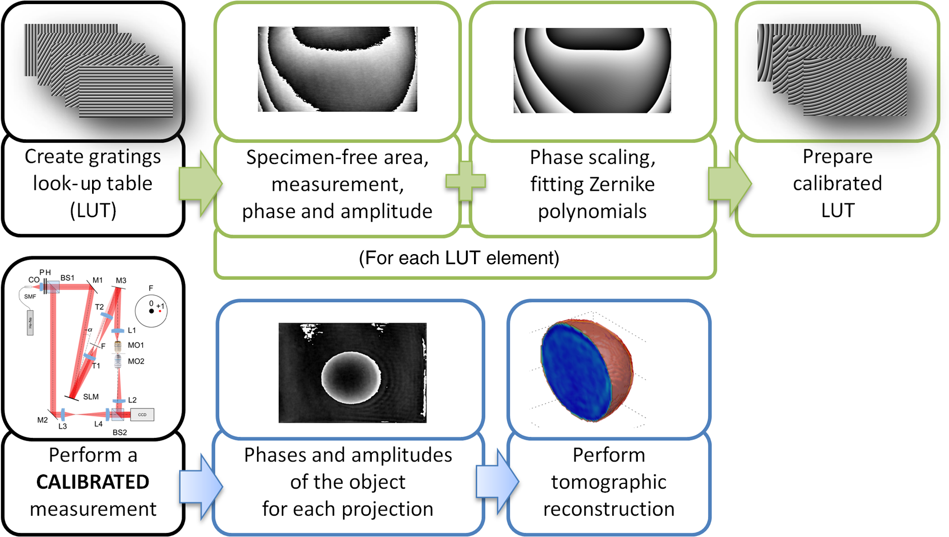
1.IntroductionFor at least a decade, quantitative phase imaging (QPI) has been a rapidly developing field of research, in which the metrological approach is introduced into biology1 as a new standard in cell studies. When it comes to setting standards, the fact that phase information has become quantitative instead of qualitative transforms observation into measurements. However, the nature of the information obtained is not the only reason to use the QPI techniques. It is the label-free, noninvasive, rapid, and high-resolution measurement capability provided by these methods2 that significantly contributes to the growing popularity of QPI in biology. The hot topics and challenges in modern cell biology cover such areas as cell life cycle, three-dimensional (3-D) position tracking, cell morphology and pathology, or even drug treatment of cancer cells. Each of the aforementioned research areas can benefit greatly from QPI and measurements, especially if the result was a 3-D refractive index distribution. Of course, the possible areas of interest for QPI can be further extended for example to cell pulsation3 and the more complete information on the phase of cells could also allow exploring cell adhesion and motility.4,5 There are a number of QPI techniques that could be used in order to investigate the biological objects in two-dimensions (2-D) as well as in 3-D. One method is the transport of intensity equation (TIE), which theoretically requires at least two images to reconstruct the phase and does not require coherent illumination.6 The fastest version of this method is the single-shot approach that can be performed by using chromatic aberration.7 This technique provides the minimum number of intensities to retrieve the phase with TIE. The acquisition of the intensities is not based on mechanical movements between planes nor does it require additional time for capturing many intensity images. Still, in some cases, more planes are obtained to increase the measurement accuracy.8 This of course increases the time of the TIE measurement. Moreover, it is not sufficient to gather more intensities and also the location of the planes should be carefully specified.9 Another interesting QPI technique providing high quality and contrast results with a limited amount of noise is ptychography.10 This method does not require a complicated optical setup; however, it does require a motorized sample stage in order to scan over the sample area, which for certain applications may not be convenient. Recently, a new approach, in which moving components were replaced with coded illumination, has been presented.11–13 Another very interesting technique in the QPI group is spatial light interference microscopy,14 which, if modified, is capable of 3-D tomographic reconstruction and is then called spatial light interference tomography (SLIT).15,16 These techniques are particularly interesting with respect to the methods described in this paper. In terms of the crucial optical components in both approaches, a spatial light modulator (SLM) and a high numerical aperture (NA) microscope objective are used. However, the SLIT tomographic reconstruction is performed in a completely different manner than in tomographic phase microscopy. The SLIT technique requires axial instead of angular scanning of the sample. Even though this is a simple operation using a motorized stage of a microscope, it is still mechanical movement and often high accuracy of the sample position is important (up to tens of nanometers). In the case of tomographic phase microscopy, as presented in this paper, mechanical scanning can be avoided in order to obtain various directions of illumination of the sample. One of the benefits of SLIT is the fact that this method uses incoherent light and therefore is not affected by the speckle noise. The method used in this paper is based on digital holographic microscopy (DHM),17 which uses interference to reconstruct the complex optical field in the sample plane. The setup for this technique may be using an object and reference beam, which is considered as a complication and a source of system instability. In principle, this may not always be an issue, since it is possible to overcome this with a common path18,19 or shearing20 configuration. A certain benefit of DHM is the capability of a single-shot measurement and the freedom of refocusing and propagating the complex optical field to different planes. However, this technique still provides only 2-D information on an integrated phase of the measured object. Furthermore, in digital holography the axial resolution is much lower than lateral. These issues may be resolved with tomographic reconstruction. In this technique, a set of holograms acquired at different viewing angles is recorded. Then, either phase or amplitude of the complex optical field, retrieved from a set of off-axis holograms, is processed with a tomographic reconstruction algorithm. This may be realized within 3-D Fourier domain, in which the Fourier transforms of the calculated images are assembled based on projection or diffraction approach.21 An alternative realization of the projection approach is to stack the phase or amplitude images and create a sinogram of the object, which is related to the 3-D reconstruction by inverse Radon transform,22 being adopted from computed tomography. The alternative realization of the sinogram-based diffraction approach requires the complex optical field propagated to the center of the object as the input. The only possible method of performing a fast measurement for holographic tomography is to illuminate the sample from different directions without rotating the object. However, in some cases, such as red blood cells membrane fluctuations analysis, the speed of the tomographic measurement may be insufficient. In this case, still, the basic DHM technique using a single projection could be used to provide a 2-D image.23 Recent research has already covered different configurations for 3-D reconstruction of refractive index or complex optical field21,24–35 as well as amplitude for fluorescent response.36 In these systems, the illumination direction is always altered mechanically using a motorized tilting mirror mounted on a stepper motor24–29 or in a much faster version using galvanometer mirrors.21,30–33 Alternatively, there has been a solution where the beam was directed using a rotating prism35 and a solution, in which a single mirror from a digital micromirror device acted as a point source.36 These solutions lead to a projection set limited by the aperture of the illumination and imaging systems; this cannot be avoided in fast tomography systems, and is also the case in the system presented in this paper. However, we propose a robust and diffraction-based method for altering the illumination angle in the limited-angle holographic tomography. Our idea of scanning is vibration-free, offers convenient point-to-point control of the illumination angle, high stability of the selected angle of illumination, and is also faster than the systems in which a mirror is mounted on a stepper motor. Additionally, it is possible to correct the wavefront error present in the specimen plane in order to provide the best quality reconstruction. Wavefront error would appear in a galvanometer-mirror-based system due to lower quality of the scanning mirrors caused by the thickness of the substrate in order to satisfy the moment of inertia requirements of the rotating mirror. Applying standard reconstruction algorithms to the data acquired with limited NA of the optical system leads to the degradation of the final result of the measurement. This is the effect of the missing information region and is especially visible in the direction of the optical axis of the measurement system.37,38 Therefore, we also developed a modified tomographic algorithm based on the total variation minimization (TVM): total variation iterative constraint (TVIC) method, which improves both external geometry and phase distribution reconstruction in the direction of optical axis as well as in the perpendicular direction. 2.Materials and Methods2.1.Experimental SetupThe tomographic microscope presented in this paper is based on a vertical setup of a holographic microscope for transparent objects in Mach–Zehnder configuration.39 This configuration is well suited for biological samples, which are usually in a liquid environment. The crucial modification of the holographic microscope is the introduction of a reflective phase-only SLM in the beam, which illuminates the object. Moreover, the system is designed in a way that additional modifications would enable integration into a DHM in the future. The scheme of the optical system of the holographic microscope is shown in Fig. 1. Fig. 1Tomographic microscope setup. He-Ne: laser; SMF: single-mode fiber; CO: collimating objective; ; P: linear polarizer; H: half-wave plate; BS1 and BS2: beam splitter cube; M1, M2, and M3: flat mirror; SLM: spatial light modulator; T1, T2, L1, L2, L3, and L4: lens; F: spatial filter; MO1: microscope objective; MO2: microscope objective; and CCD: charge coupled device camera.  The He-Ne laser beam () is delivered to the setup using a polarization-maintaining, single-mode fiber and is then collimated with a 100-mm focal length lens. The polarizer and half-wave plate (multiorder plate, designed for ) are used to control the intensity and the azimuth of polarization required for the phase-only liquid crystal (LC) SLM to work with. Then, the beam is split into reference and object beams by a 50:50 beam-splitting cube. The reference beam is directed by the M2 mirror toward the CCD. It passes through a beam expander, which consists of L3 () and L4 (). This component is useful for introducing a spatial carrier in the holograms. The object beam is directed through the M1 mirror toward the high-resolution ( pixels, pixel pitch, 93% fill factor) liquid crystal on silicon (LCoS) SLM, PLUTO-VIS-014 (Holoeye Photonics AG, Germany). The beam impinges on the SLM at the angle— equal to 8 deg. The SLM is placed in the front focal plane (FFPL) of the T1 lens (). The T2 lens () acts as a second lens of the (T1–T2) telescope system. The spatial filter , which is used to block zero diffraction order and reflection from the SLM cover glass, is optional. The image of the SLM surface is created in the back focal plane (BFPL) of the L1 lens (). The beam is focused in the FFPL of the MO1 microscope objective (Olympus UPlanFLN , infinity-corrected, 0.17 CS—cover slip, ). If a blazed grating is displayed on the modulator, the incident plane wave is diffracted into a single diffraction order. Expanded by the telescope, the diffracted beam is focused in the FFPL of the MO1 objective and creates a tilted illumination of the sample. When a series of blazed gratings with controlled frequency and direction is displayed on the modulator, the FFPL of the MO1 is scanned (see Sec. 3). Each point in the FFPL corresponds to an inclined beam in the specimen plane. Imaging of the sample illuminated in this manner is performed using the MO2 microscope objective (Leica HCX Pl APO to 0.75 CS, ). The plane wave, illuminating the sample, is focused in the BFPL of the MO2 and collimated using the L2 tube lens (). The CCD camera (JAI BM-500GE, pixels, pixel size) is placed in the BFPL of the L2 lens. The magnification of the imaging part of the system is 38. In this tomographic microscope, the SLM replaces two rotary mirrors, which would normally be necessary to scan the aperture of the MO1 microscope objective. Implementing SLM as an active element for scanning directions of the object-illuminating beam provides the freedom of different illumination scenarios. Below, we describe two basic types of illumination scenarios: linear and circular. In the case presented in Fig. 2(a), a spatial filter (Fig. 1) is placed in the Fourier plane of the T1 lens. Scanning the aperture of the MO1 along a circle results in illumination beams lying on a cone. In this approach, the frequency of the spatial carrier rotating in the camera plane is constant for each projection, which is beneficial for hologram processing. In the scanning method presented in Fig. 2(b), the illumination beams lie in one plane. This concept allows capturing an image for normal illumination. Here, the spatial carrier frequency is no longer constant, which might lead to issues with too low or too high fringe density. Fig. 2Basic illumination scenarios in tomographic measurement presented in the image plane, (a) the result of circular scanning of the back focal plane (BFPL) of the MO1 microscope objective with object beam, : ’th sample wave vector, to total number of projections, : reference beam, : maximum sample beam incidence angle in the image plane, : azimuth of the ’th projection, (b) the result linear scanning of the BFPL of the MO1 objective, : reference beam angle of incidence in the camera plane.  The results of data acquisition are presented in Fig. 3. The spatial carrier frequency in Figs. 3(a) and 3(b) depends on the illumination angle only and for Fig. 3(c) can also be adjusted with angle (with a single, mechanical tilt of the M2 mirror) to obtain optimal conditions for phase reconstruction for every projection. The spatial carrier frequency should not exceed the Nyquist limit for . Fig. 3Off-axis holograms of a PMMA microsphere: (a) circular scanning measurement (CSM) scenario, angle of incidence of the illumination beam in the specimen plane , , , (b) CSM scenario, angle of incidence of the illumination beam in the specimen plane , , , and (c) linear scanning measurement (LSM) scenario, .  2.2.Spatial Light Modulator as an Active Device in Tomographic Microscope2.2.1.Beam steeringThe main function of the SLM in the tomographic microscope is a vibration-free, diffraction-based beam deflection, which is used to acquire a set of holograms for a series of illumination angles. For this purpose, a series of blazed gratings is displayed on the SLM. For the circular illumination scenario, the blazed grating is rotated in the SLM plane; for the linear scenario, the period of the grating is varied for each projection. However, several conditions and limitations of SLMs need to be considered and taken into account to obtain illumination distribution that would allow a high-quality tomographic reconstruction. Apart from the accuracy and the quality of the holograms, the quality of the reconstruction depends strongly on the angular span of the projections, which should be as large as possible, and the number of the projections, which should also be maximized. Unfortunately, the SLM can only display blaze steps with width equal to -times pixel size (), which limits the period of the displayed grating and maximum diffraction angle to 2.27 deg (). However, should the measurement system have optimum energy efficiency, the minimum period of a blazed grating is further limited to (diffraction efficiency for the -1st order40). Thus, the smallest period of the blazed grating displayed on the SLM should be equal to , which corresponds to 0.57 deg of the diffraction angle. On the other hand, the maximum possible illumination angle is in this case limited by the NA of the MO2 objective and the refractive index of the immersion medium (), which means that . This imposes the minimal angular magnification of the T1-T2-L1-MO1 part of the system. However, even if this is taken into account, the angle of illumination in the sample plane is not linearly dependent on the blaze width. This means that in the systems, which have angular magnification of the telescopes around , near the , a sample can be illuminated every 4 deg and the cut-off illumination angle is 1 deg. The normal illumination is realized when no grating is displayed on the modulator. It is possible to increase linearity and decrease angular step near the maximum illumination angle if the angular magnification () of the telescopes is increased. In our system, we propose the . The minimum blazed grating period used is 15 pixels, which corresponds to incidence angle in the sample plane. In a linear scanning scenario, the cut-off illumination angle is 1 deg and the angular step near is equal to 2 deg. This nonuniform distribution will be taken into account in the tomographic reconstruction. This is not a problem with circular scanning, which is based on rotating a 15 pixel blazed grating at 1 deg interval. In the linear scanning scenario, there were 265 holograms acquired with angular step of 0.2 to 2 deg. For the circular scanning scenario, there were 360 holograms captured at one degree of rotation intervals, at . Finally, the measurement speed with an SLM is limited by the refresh rate of the phase microdisplay, which is 60 Hz. However, in order to avoid display errors, the maximum achievable frame rate of the display would have to be limited at least by half (toggle rate). In this particular case, the displaying rate was limited by the software efficiency (Java full-screen display procedures run by MATLAB) to 11 Hz. Currently, the optical beam steering does not match the performance of galvanometer-mirror-based systems, in which the top speed of data acquisition is 150 times higher;31 however, it is possible to increase the speed of the system using a 500 Hz SLM. 2.2.2.Wavefront correctionSLMs are common tools in wavefront correction41,42 and are also used in microscopy to improve image quality.43 Phase-only, reflective modulators are also used in interferometry for wavefront shaping.44 In this case, the correction of the object beam wavefront compensates for the shape of the SLM, which is not perfectly flat, and the aberration that is present at angles close to . Also, if a biological sample was measured, the refractive index mismatch between the immersion liquid and the specimen would result in spherical aberration. In this approach, the calibration is a convenient procedure because it is only necessary to find a sample-free region and create a look-up table (LUT) once per measurement scenario and a sample with specific refractive index. In this paper, to display a phase image for wavefront correction, Zernike orthogonal polynomials45 are used to fully characterize the aberrations. SLM is rectangular, therefore it is important that the polynomials are calculated over a rectangular aperture46 instead of a unit disk. In this work, the first 15 Noll indices of the polynomials were used. Processing the reference image to calculate correction map could of course also be realized using averaging, filtering methods such as bidimensional empirical mode decomposition47 or alternative image reconstruction technique based on orthogonal moments.48 However, the established theory for calculating the wavefront aberrations based on the Zernike polynomials of the reference measurement appears to be the most functional approach for wavefront correction. The pixel size of the modulator is , while the camera pixel size is . The basic condition for reconstructing the wavefront for the SLM with a camera used for imaging is to maintain the relation . In the case presented here, in the camera plane is , which means that the resolution of the SLM is not fully used in wavefront correction and additional errors may occur during the processing of the reference wavefront map. The result of the calculation of the Zernike-polynomials-based wavefront map for the SLM is presented in Fig. 4. Calculation of the wavefront map does not take into account the higher frequencies in the phase. In this way, the calibration is not affected by the noise introduced by the sample-free area and only corrects aberration introduced by the optical system and the shape of the modulator. Fig. 4Wrapped correction phase for illumination angle: (a) the reference wavefront and (b) wavefront reconstructed from calculated Zernike polynomials for coefficients 1 to 15th Noll index.  The benefit from correcting the wavefront is the fact that the quality of the reconstructed image is improved. Moreover, the sample does not need to be removed in order to place a calibration object, which is convenient. Also, when multiple objects are measured within one sample chamber, the processing of the phase images is simplified—there is no need to subtract the background wavefront or perform additional deconvolution operations. 2.3.Measurement ProcedureIn order to perform calibration and measurement using the active tomographic microscope with optically controlled projections, a few steps must be performed. This is shown briefly in Fig. 5. In the approach presented in this paper, the preprocessing part of the measurement is extended. The key part of the preprocessing is calculating Zernike polynomials followed by preparation of calibrated LUT containing a blazed grating for each projection. The effect of the superposition of the correction wavefront and the blazed grating is presented in Fig. 6. The maximum intensity of the created pattern is adjusted to match the required phase shift. Fig. 6An example of a LUT frame for a 36-pixel blazed grating (): (a) precalibration blazed grating and (b) calibrated LUT frame, modified with reference wavefront.  The result of implementation of the regular and corrected LUT cells is presented in Fig. 7. The wavefront has been successfully corrected over the sample area and most of the SLM. It can be noticed that errors caused by the borders of the SLM are not corrected well. In addition, apparently the correction wavefront might not fully match the real aberrated wavefront. This might occur if the SLM border is not perfectly parallel to the camera plane. For this reason, a calibration method needs to be proposed in the future. Also, placing an amplitude mask in the plane conjugate with the SLM surface would reduce the diffraction caused by the border of the modulator. 2.4.Tomographic ReconstructionThe illumination architectures described above do not provide data from full tomographic angular range and therefore require a special approach. According to the diffraction slice theorem, these architectures result in empty areas in the Fourier domain,21 which in turn strongly influence reconstruction resolution, which becomes anisotropic. Anisotropic resolution is not the only artifact present in the reconstruction. Another is a distorted geometry of the reconstructed object—the shape is elongated in the direction in which no projections were recorded.37,38 In general, the problem of tomographic reconstruction becomes even more problematic, which in this case means that from the same set of initial data, an almost infinitely large set of solutions with a relatively small residuum may be calculated.49 A number of algorithms that compensate for the partial lack of input data have already been developed.50 The state-of-the-art approaches utilize TVM,51–54 a technique derived from compressed sensing. TV minimization is a very powerful regularizer that makes use of the fact that some objects’ gradient is sparse. By applying the TVM iteratively in the reconstruction process, one can limit the number of possible solutions of the tomographic reconstruction, thus it is possible to retrieve full information about the object. By definition, the TVM is applicable to piecewise constant samples only. Herein, we propose a novel technique, namely the TVIC. It allows applying the TVM technique to reconstruct nonpiecewise constant samples such as biological cells. In this approach, in the first step, a piecewise constant reconstruction of the sample is calculated by means of Chambolle–Pock algorithm.55 Despite the fact that inner structures of the reconstructed sample are erroneous (by applying Chambolle–Pock algorithm we assumed piecewise constancy to a nonpiecewise constant specimen), the external geometry is retrieved correctly with very good precision. This reconstruction is binarized and treated as an external geometry mask. The knowledge about external geometry is now a powerful prior, which strongly improves the final results. In our approach, this prior is applied iteratively to the algebraic reconstruction algorithm.56 Other priors are nonnegativity constraint and smoothness of the refractive index distribution. The latter prior is implemented in the form of a 3-D median filter of the size. When algebraic reconstruction techniques are applied to 3-D tomography, the size of the system matrix from the equation , in which is the reconstructed image and is the input data (sinogram), is always a problem. In our case, the system matrix has a size of approximately , which would normally mean more than 10 TB of data. This is why we utilize the ASTRA Toolbox,57 which makes use of the fact that a major part of this matrix consists of zeros and so the matrix may be created with a reasonable amount of memory. It also allows the implementation of custom TV regularizers. The algorithm results in a reconstruction with partially improved quality of inner structures of the specimen and with precisely retrieved external geometry. During the main reconstruction stage, the piecewise constancy was not assumed, making it applicable to a wide range of samples. 2.5.Sample PreparationOne of the two samples prepared for the experiment in this paper was a microsphere made of PMMA. The microspheres were produced by microParticles GmbH. The diameter of the sphere was and the refractive index for is , and it was immersed in index-matching liquid (Cargille) with refractive index . The object was placed between two 0.17 mm coverslips separated with #0 coverslip (0.08-mm thick). As the second sample, the C2C12 mouse myoblast cell line58 was prepared. The C2C12 cells were maintained in DMEM high glucose medium with l-glutamine and sodium pyruvate (Gibco) supplemented with 10% fetal bovine serum (Sigma–Aldrich) and 1% penicillin/streptomycin mixture (Life Technologies) at 37°C in a humidified 95% air and 5% atmosphere. Cells were passaged at 70% to 80% of confluence. For the experiment, cells were seeded on autoclaved 0.17 mm coverslips. Cells on coverslips were rinsed briefly with cold phosphate buffer saline (PBS) (Pracownia Chemii Ogólnej IIITD PAN) and fixed in 4% paraformaldehyde (Sigma–Aldrich) for 10 min at room temperature. Next, the coverslips were rinsed with cold PBS buffer ( at room temperature). Finally, the coverslips were stored in PBS buffer supplemented with 0.02% sodium azide (Sigma–Aldrich). For the measurement, coverslips with cells were supported on two #0 coverslip spacers and covered with a #1 coverslip. For the measurement, the cells were immersed in water ( at and ). 3.Results3.1.Tomographic Reconstruction of a Calibrated ModelIn order to test the performance of the algorithm as well as compare the proposed scanning scenarios, a well–defined object, i.e., polymer microsphere, was measured. Two illumination architectures were used in the measurement, as described in Sec. 2.1: single-axis (linear) illumination and conical illumination. The acquired data were reconstructed with TVIC algorithm. It should be noted that the calibrated object is piecewise constant, but during the second stage of the reconstruction process piecewise constancy was not assumed. However, the piecewise constant microsphere still allows verification of the quality of the reconstruction in terms of shape and refractive index changes. Figures 8 and 9 present the reconstruction of the refractive index distribution in the microsphere based on the data captured with the single-axis illumination and the conical illumination scenarios, respectively. The color scale represents the absolute refractive index values calculated using the a priori information of the refractive index of the background (certified index-matching liquid). Fig. 8Central cross section of a three-dimensional (3-D) reconstruction of the refractive index of a microsphere reconstructed from data gathered using the linear illumination scanning measurement scenario.  Fig. 9Central cross section of a 3-D reconstruction of refractive index of the microsphere reconstructed from data gathered using the CSM scenario.  Figures 8 and 9 show that TVIC algorithm provides correct external geometry of the measured object. There is also visible improvement in the reconstruction of the inner structure when these results are compared with results calculated with SART+ATV algorithm.26,37 However, it is clearly visible in Fig. 8(b) that the shape of the microsphere obtained with LSM is distorted along the direction of the optical axis, which is even more apparent in Fig. 10(a). Fig. 10The comparison of the microsphere 3-D refractive index distribution reconstruction profiles in two directions ( and ) for (a) LSM scenario and (b) CSM scenario.  The asymmetry of the microsphere measured with the circular scanning scenario (along the - and -axes) is in this case less than 1.7% with a slight elongation of the reconstruction in the direction of optical axis. We consider this to be a very good result and, based on this, have decided to use only a CSM scenario. Also, the distribution of the refractive index in the direction is much more uniform and similar to the profile for the circular scanning measurement. In the case of the linear measurement, the inner structure of the microsphere was affected by the character of scanning and could be reduced if the linear scanning was performed in two directions. The reconstructed value of the refractive index in the center of the PMMA microsphere lies within the uncertainty usually estimated for limited-angle tomographic systems.32 3.2.Tomographic Reconstruction of a Biological SampleIn this section, we present the second step of the experiment, in which fixed adherent cells from the C2C12 line were measured. Even though we did not measure living biological samples, our technique is equally suitable for such objects. The result of the measurement is shown in Fig. 11. In the reconstruction slices presented in Fig. 11(b), the region of highest refractive index values can be identified as the nucleus of the C2C12 cell, and the nuclear envelope is visible. The regions of higher refractive index in the nucleus are also visible, which could correspond to the nucleoli. We find our result to be in agreement with DHM-based studies on the refractive index of the intracellular structures of adherent cells.59 Fig. 11Tomographic reconstruction of a single C2C12 cell, measured using the CSM scenario and scaled to absolute refractive index values: (a) slice through the sample in the specimen plane (), (b) slice through the sample containing the optical axis (), (c) slice in 3-D (Video 1, MPEG, 1.4 MB) [URL: http://dx.doi.org/10.1117/1.JBO.20.11.111216.1], and (d) slice in 3-D.  The reconstructed cell example is artifact free and does not exhibit any significant error at the borders, which suggests that the algorithm performs better for nonpiecewise constant objects than the piecewise constant calibration object. However, to fully characterize the reconstruction quality and accuracy, a well-defined 3-D phase phantom would be very useful. 4.ConclusionIn this paper, new approaches to the projection generation in the holographic tomography measurement system and to the reconstruction using a limited set of projections were demonstrated. Placing an SLM in the tomographic microscope allows a vibration-free and robust operation. The optically controlled illumination angle is a convenient solution, due to the illumination scenarios it enables, which could be adjusted according to the measured object type. In addition, the SLM allows wavefront correction. This is an interesting feature, because although it is possible to numerically process the obtained phase images using propagation techniques or numerical aberration correction, the illuminating wavefront correction is not possible in this way. In the future, the performance of the wavefront correction should be verified and thoroughly tested. The algorithm proposed in the paper was proved to enhance the quality of the limited-angle reconstruction and extends the number of object types that can be successfully reconstructed to nonpiecewise constant samples, such as biological objects, e.g., cancer cells. It should be noted that tomographic studies of a calibrated object32 usually do not focus on the quality of the slices at planes containing the optical axis, e.g., and planes, since it is much easier to supplement the missing region of data in the Fourier domain in and directions than in .38 Improving the reconstruction in the direction of the optical axis while maintaining the correct reconstruction in the perpendicular direction was the main challenge of the reconstruction algorithm demonstrated in this paper; based on the calibrated object results, we claim this to be a success. In the future, the method presented here should be implemented for the diffraction-based approach, which could lead to an improvement. Furthermore, in this paper only two basic measurement scenarios were tested. It would be beneficial to thoroughly analyze different possible sample illumination scenarios and determine the minimum number of projections and the optimum distribution of the scanning points in the focal plane of the illumination objective. AcknowledgmentsThe research leading to the described results are realized within the program TEAM/2011-7/7 of Foundation for Polish Science, cofinanced from the European Funds of Regional Development. The authors would like to acknowledge the support from the grant of the Dean of Mechatronics Faculty, Warsaw University of Technology. Networking support was provided by the EXTREMA COST Action MP1207. We would like to thank Folkert Bleichrodt and Tristan van Leeuwen for providing the code for the Chambolle–Pock algorithm and Dr. Tytus Bernaś and Natalia Nowak from Laboratory of Imaging Tissue Structure and Function, Nencki Institute of Experimental Biology for providing biological samples. ReferencesT. Kim et al.,
“Breakthroughs in photonics 2013: quantitative phase imaging: metrology meets biology,”
IEEE Photonics J., 6 1
–9
(2014). http://dx.doi.org/10.1109/JPHOT.2014.2309647 Google Scholar
K. Lee et al.,
“Quantitative phase imaging techniques for the study of cell pathophysiology: from principles to applications,”
Sensors (Basel), 13 4170
–4191
(2013). http://dx.doi.org/10.3390/s130404170 Google Scholar
O. J. Pletjushkina et al.,
“Induction of cortical oscillations in spreading cells by depolymerization of microtubules,”
Cell Motil. Cytoskeleton, 48 235
–244
(2001). http://dx.doi.org/10.1002/cm.1012 CMCYEO 0886-1544 Google Scholar
P. Pomorski et al.,
“How adhesion, migration, and cytoplasmic calcium transients influence interleukin-1β mRNA stabilization in human monocytes,”
Cell Motil. Cytoskeleton, 57 143
–157
(2004). http://dx.doi.org/10.1002/cm.10159 CMCYEO 0886-1544 Google Scholar
P. Roy et al.,
“Microscope-based techniques to study cell adhesion and migration,”
Nat. Cell Biol., 4
(4), E91
–E96
(2002). http://dx.doi.org/10.1038/ncb0402-e91 Google Scholar
J. C. Petruccelli, L. Tian and G. Barbastathis,
“The transport of intensity equation for optical path length recovery using partially coherent illumination,”
Opt. Express, 21 14430
–14441
(2013). http://dx.doi.org/10.1364/OE.21.014430 OPEXFF 1094-4087 Google Scholar
L. Waller et al.,
“Phase from chromatic aberrations,”
Opt. Express, 18
(22), 22817
–22825
(2010). http://dx.doi.org/10.1364/OE.18.022817 OPEXFF 1094-4087 Google Scholar
L. Waller, L. Tian and G. Barbastathis,
“Transport of intensity phase-amplitude imaging with higher order intensity derivatives,”
Opt. Express, 18 12552
–12561
(2010). http://dx.doi.org/10.1364/OE.18.012552 OPEXFF 1094-4087 Google Scholar
J. Martinez-Carranza, K. Falaggis and T. Kozacki,
“Optimum plane selection for transport-of-intensity-equation-based solvers,”
Appl. Opt., 53
(50), 7050
–7058
(2014). http://dx.doi.org/10.1364/AO.53.007050 APOPAI 0003-6935 Google Scholar
J. Marrison et al.,
“Ptychography-a label free, high-contrast imaging technique for live cells using quantitative phase information,”
Sci. Rep., 3 2369
(2013). http://dx.doi.org/10.1038/srep02369 SRCEC3 2045-2322 Google Scholar
L. Tian et al.,
“Multiplexed coded illumination for Fourier ptychography with an LED array microscope,”
Biomed. Opt. Express, 5 2376
–2389
(2014). http://dx.doi.org/10.1364/BOE.5.002376 BOEICL 2156-7085 Google Scholar
X. Ou et al.,
“High numerical aperture Fourier ptychography: principle, implementation and characterization,”
Opt. Express, 23
(3), 3472
(2015). http://dx.doi.org/10.1364/OE.23.003472 OPEXFF 1094-4087 Google Scholar
L. Tian and L. Waller,
“3D intensity and phase imaging from light field measurements in an LED array microscope,”
Optica, 2 104
–111
(2015). http://dx.doi.org/10.1364/OPTICA.2.000104 Google Scholar
Z. Wang et al.,
“Spatial light interference microscopy (SLIM),”
Opt. Express, 19
(2), 1016
–1026
(2011). http://dx.doi.org/10.1364/OE.19.001016 OPEXFF 1094-4087 Google Scholar
M. Mir et al.,
“Visualizing Escherichia coli sub-cellular structure using sparse deconvolution spatial light interference tomography,”
PLoS One, 7
(6), e38916
(2012). http://dx.doi.org/10.1371/journal.pone.0039816 POLNCL 1932-6203 Google Scholar
T. Kim et al.,
“White-light diffraction tomography of unlabelled live cells,”
Nat. Photonics, 8 256
–263
(2014). http://dx.doi.org/10.1038/nphoton.2013.350 NPAHBY 1749-4885 Google Scholar
K. Alm et al.,
“Cells and holograms–holograms and digital holographic microscopy as a tool to study the morphology of living cells,”
Holography—Basic Principles and Contemporary Applications, In Tech, Rijeka, HR
(2013). http://dx.doi.org/10.5772/46111 Google Scholar
K. Kim et al.,
“Diffraction optical tomography using a quantitative phase imaging unit,”
Opt. Lett., 39
(24), 6935
–6938
(2014). http://dx.doi.org/10.1364/OL.39.006935 OPLEDP 0146-9592 Google Scholar
K. Lee and Y. Park,
“Quantitative phase imaging unit,”
Opt. Lett., 39 3630
–3633
(2014). http://dx.doi.org/10.1364/OL.39.003630 OPLEDP 0146-9592 Google Scholar
G. G. Levin et al.,
“Shearing interference microscopy for tomography of living cells,”
Proc. SPIE, 9536 95360G
(2015). http://dx.doi.org/10.1117/12.2183717 PSISDG 0277-786X Google Scholar
K. Kim et al.,
“High-resolution three-dimensional imaging of red blood cells parasitized by Plasmodium falciparum and in situ hemozoin crystals using optical diffraction tomography,”
J. Biomed. Opt., 19 011005
(2014). http://dx.doi.org/10.1117/1.JBO.19.1.011005 JBOPFO 1083-3668 Google Scholar
A. Kak and M. Slaney, Principles of Computerized Tomographic Imaging, IEEE Press, New York
(1988). Google Scholar
Y. Kim et al.,
“Profiling individual human red blood cells using common-path diffraction optical tomography,”
Sci. Rep., 4 6659
(2014). http://dx.doi.org/10.1038/srep06659 SRCEC3 2045-2322 Google Scholar
V. Lauer,
“New approach to optical diffraction tomography yielding a vector equation of diffraction tomography and a novel tomographic microscope,”
J. Microsc., 205 165
–176
(2002). http://dx.doi.org/10.1046/j.0022-2720.2001.00980.x JMICAR 0022-2720 Google Scholar
M. Debailleul et al.,
“Holographic microscopy and diffractive microtomography of transparent samples,”
Meas. Sci. Technol., 19 074009
(2008). http://dx.doi.org/10.1088/0957-0233/19/7/074009 MSTCEP 0957-0233 Google Scholar
A. Kus et al.,
“Limited-angle hybrid diffraction tomography for biological samples,”
Proc. SPIE, 9132 91320O
(2014). http://dx.doi.org/10.1117/12.2051973 PSISDG 0277-786X Google Scholar
A. Barty et al.,
“Quantitative phase tomography,”
Opt. Commun., 175 329
(2000). http://dx.doi.org/10.1016/S0030-4018(99)00726-9 OPCOB8 0030-4018 Google Scholar
B. Simon et al.,
“High-resolution tomographic diffractive microscopy of biological samples,”
J. Biophotonics, 3 462
–467
(2010). http://dx.doi.org/10.1002/jbio.200900094 Google Scholar
M. Debailleul et al.,
“Diffractive microscopy of transparent inorganic and biological samples,”
Opt. Lett., 34 79
–81
(2009). http://dx.doi.org/10.1364/OL.34.000079 Google Scholar
W. Choi et al.,
“Tomographic phase microscopy,”
Nat. Methods, 4 717
–719
(2007). http://dx.doi.org/10.1038/nmeth1078 1548-7091 Google Scholar
C. Fang-Yen et al.,
“Video-rate tomographic phase microscopy,”
J. Biomed. Opt., 16 011005
(2011). http://dx.doi.org/10.1117/1.3522506 JBOPFO 1083-3668 Google Scholar
Y. Sung et al.,
“Optical diffraction tomography for high resolution live cell imaging,”
Opt. Express, 17
(1), 266
(2009). http://dx.doi.org/10.1364/OE.17.000266 OPEXFF 1094-4087 Google Scholar
P. Xiu et al.,
“Controllable tomography phase microscopy,”
Opt. Lasers Eng., 66 301
–306
(2015). http://dx.doi.org/10.1016/j.optlaseng.2014.10.001 Google Scholar
M. Debailleul et al.,
“High-resolution three-dimensional tomographic diffractive microscopy of transparent inorganic and biological samples,”
Opt. Lett., 34
(1), 79
–81
(2009). http://dx.doi.org/10.1364/OL.34.000079 OPLEDP 0146-9592 Google Scholar
Y. Cotte et al.,
“Marker-free phase nanoscopy,”
Nat. Photonics, 7 113
–117
(2013). http://dx.doi.org/10.1038/nphoton.2012.329 NPAHBY 1749-4885 Google Scholar
R. Chamgoulov, P. Lane and C. MacAulay,
“Optical computed-tomography microscope using digital spatial light modulation,”
Proc. SPIE, 5324 182
–190
(2004). http://dx.doi.org/10.1117/12.526903 PSISDG 0277-786X Google Scholar
W. Krauze, A. Kus and M. Kujawinska,
“Limited-angle hybrid optical diffraction tomography system with total-variation-minimization-based reconstruction,”
Opt. Eng., 54 054104
(2015). http://dx.doi.org/10.1117/1.OE.54.5.054104 Google Scholar
J. Lim et al.,
“Comparative study of iterative reconstruction algorithms for missing cone problems in optical diffraction tomography,”
Opt. Express, 23
(13), 16933
(2015). http://dx.doi.org/10.1364/OE.23.016933 OPEXFF 1094-4087 Google Scholar
B. Rappaz et al.,
“Digital holographic microscopy: a quantitative label-free microscopy technique for phenotypic screening,”
Comb. Chem. High Throughput Screening, 17 80
–88
(2014). http://dx.doi.org/10.2174/13862073113166660062 CCHSFU 1386-2073 Google Scholar
S. Sinzinger and J. Jahns, Microoptics, 168 Wiley-VCH, Weinheim, DE
(2003). Google Scholar
J. Arines et al.,
“Measurement and compensation of optical aberrations using a single spatial light modulator,”
Opt. Express, 15
(23), 15287
–15292
(2007). http://dx.doi.org/10.1364/OE.15.015287 OPEXFF 1094-4087 Google Scholar
J. Zhang et al.,
“Wave front transformation and correction by using SLM,”
Proc. SPIE, 6711 67110C
(2007). http://dx.doi.org/10.1117/12.731960 PSISDG 0277-786X Google Scholar
O. Azucena et al.,
“Implementation of adaptive optics in fluorescent microscopy using wavefront sensing and correction,”
Proc. SPIE, 7595 75950I
(2010). http://dx.doi.org/10.1117/12.846380 PSISDG 0277-786X Google Scholar
J. Kacperski and M. Kujawinska,
“Phase only SLM as a reference element in Twyman–Green laser interferometer for MEMS measurement,”
Proc. SPIE, 6616 66163E
(2007). http://dx.doi.org/10.1117/12.726214 PSISDG 0277-786X Google Scholar
F. Zernike,
“Beugungstheorie des Schneidenverfahrens und Seiner Verbesserten Form, der Phasenkontrastmethode,”
Physica, 1
(8), 689
–704
(1934). http://dx.doi.org/10.1016/S0031-8914(34)80259-5 Google Scholar
V. N. Mahajan and G.-M. Dai,
“Orthonormal polynomials in wavefront analysis: analytical solution,”
J. Opt. Soc. Am. A, 24
(9), 2994
–3016
(2007). http://dx.doi.org/10.1364/JOSAA.24.002994 JOAOD6 0740-3232 Google Scholar
M. Trusiak, M. Wielgus and K. Patorski,
“Advanced processing of optical fringe patterns by automated selective reconstruction and enhanced fast empirical mode decomposition,”
Opt. Laser Eng., 52 230
–240
(2014). http://dx.doi.org/10.1016/j.optlaseng.2013.06.003 OLENDN 0143-8166 Google Scholar
B. Bayraktar et al.,
“A numerical recipe for accurate image reconstruction from discrete orthogonal moments,”
Pattern Recognit., 40
(2), 659
–669
(2007). http://dx.doi.org/10.1016/j.patcog.2006.03.009 Google Scholar
P. C. Hansen, Discrete Inverse Problems: Insight and Algorithms, SIAM-Society for Industrial and Applied Mathematics, Pennsylvania, PA
(2010). Google Scholar
D. Verhoeven,
“Limited-data computed tomography algorithms for the physical sciences,”
Appl. Opt., 32
(20), 3736
–3754
(1993). http://dx.doi.org/10.1364/AO.32.003736 APOPAI 0003-6935 Google Scholar
M. Ertas et al.,
“Digital breast tomosynthesis image reconstruction using 2D and 3D total variation minimization,”
Biomed. Eng. Online, 12 112
(2013). http://dx.doi.org/10.1186/1475-925X-12-112 Google Scholar
M. Burger et al.,
“Total variation regularisation in measurement and image space for PET reconstruction,”
Numer. Anal. Inverse Problems, 30
(10), 1
–30
(2014). http://dx.doi.org/10.1088/0266-5611/30/10/105003 Google Scholar
X. Jin et al.,
“Anisotropic total variation for limited-angle CT reconstruction,”
in IEEE Nuclear Science Symp. & Medical Imaging Conf.,
2232
–2238
(2010). Google Scholar
D. Chen et al.,
“The properties of SIRT, TVM, and DART for 3D imaging of tubular domains in nanocomposite thin-films and sections,”
Ultramicroscopy, 147 137
–148
(2014). http://dx.doi.org/10.1016/j.ultramic.2014.08.005 ULTRD6 0304-3991 Google Scholar
A. Chambolle and T. Pock,
“A first-order primal–dual algorithm for convex problems with applications to imaging,”
J. Math. Imaging Vision, 40
(1), 120
–145
(2011). http://dx.doi.org/10.1007/s10851-010-0251-1 Google Scholar
A. Andersen,
“Simultaneous algebraic reconstruction technique (SART): a superior implementation of the ART algorithm,”
Ultrasonic Imaging, 6
(1), 81
–94
(1984). http://dx.doi.org/10.1177/016173468400600107 ULIMD4 0161-7346 Google Scholar
W. J. Palenstijn, K. J. Batenburg and J. Sijbers,
“Performance improvements for iterative electron tomography reconstruction using graphics processing units (GPUs),”
J. Struct. Biol., 176
(2), 250
–253
(2011). http://dx.doi.org/10.1016/j.jsb.2011.07.017 JSBIEM 1047-8477 Google Scholar
D. Yaffe and O. Saxel,
“Serial passaging and differentiation of myogenic cells isolated from dystrophic mouse muscle,”
Nature, 270
(5639), 725
–727
(1977). http://dx.doi.org/10.1038/270725a0 Google Scholar
S. Przibilla,
“Sensing dynamic cytoplasm refractive index changes of adherent cells with quantitative phase microscopy using incorporated microspheres as optical probes,”
J. Biomed. Opt., 17 097001
(2012). http://dx.doi.org/10.1117/1.JBO.17.9.097001 JBOPFO 1083-3668 Google Scholar
BiographyArkadiusz Kuś is a PhD student at the Warsaw University of Technology. He received his MSc Eng degree in automation and robotics with specialization in photonics engineering from Warsaw University of Technology, Faculty of Mechatronics, in 2011. Apart from his scientific career, he also worked for the company PZO Microscopes and Optical Devices, Ltd., located in Warsaw, Poland. His current research interests include optical diffraction tomography, holography, and optical design. Wojciech Krauze graduated from Warsaw University of Technology in 2013, where he studied photonics engineering in the Mechatronics Department and where he received his MSc degree. Currently, he is studying his PhD course at the Warsaw University of Technology. His main research tasks include developing algorithms for limited-angle tomography and new noninvasive methods for analysis of biological samples. Małgorzata Kujawińska is a fellow of SPIE, a full professor of applied optics at the Warsaw University of Technology, and a head of the Photonics Engineering Division at the Institute of Micromechanics and Photonics. She is an expert in full-field optical metrology, hybrid optonumerical methods in mechanics, image processing, automatic data analysis, and design of novel photonics systems. Since 1980 she has been involved in optical metrology topics including development of interferometric, holographic, grating interferometry, diffraction tomography, digital image correlation, and structured light based methods. She is the author of one monograph, several book chapters, and more than 200 papers in international scientific journals. |