1.

Introduction

Cancer is a disease of uncontrolled cell growth, beginning with one cell or a small group of cells, spreading over to different organs, and ultimately causing death if not controlled. According to GLOBOCAN fact sheet 2012, cancer-related mortality accounts for 8.2 million worldwide, out of which breast cancer alone accounts for 0.52 million.¹ Breast cancer begins as a premalignant disease and reaches to its advanced and/or metastatic stage through various phases of tumor progression. The nonmodifiable factors responsible for breast cancer are the female gender itself, age, BRCA1 and BRCA2 genes, and personal factors such as a long menstrual history, use of oral contraceptives, and having first child after age 30 or nulliparous.² Among the modifiable factors, the major risks are being overweight, lifestyle, taking hormone replacement therapy, taking birth control pills, drinking alcohol, having tobacco, etc. Once a breast tumor is developed, its growth and progression are always supported by the surrounding tumor microenvironment. It is supposed to be composed of a variety of cell types including endothelial cells, pericytes, smooth-muscle cells, fibroblasts of various phenotypes, myofibroblasts, immune cells, natural killer lymphocytes, and antigen-presenting cells, such as macrophages and also dendritic cells. They are often characterized by conditions like hypoxia, nutrient deprivation, acidosis, abnormal tumor angiogenesis, aberrant stroma, etc.^3,4 There are several proteins secreted during the progression of the disease. These proteins play a key role in the biological pathway leading to the development and prognosis of the disease. The identification and characterization of these proteins (biomarkers) may lead to a better understanding of the disease patterns. However, the heterogeneous nature of breast cancer makes biomarker identification a challenging task and alternative strategies are needed to address this problem by detecting the cancer early.

The current available techniques for breast cancer detection are clinical breast exam, mammography, ultrasounds, molecular breast imaging, and magnetic resonance imaging (MRI), especially for women with a high risk of breast cancer.⁵ Mammography and ultrasonography are considered to be the most effective screening techniques for the premenopausal and postmenopausal women, respectively.⁶ Besides their applicability, these techniques have some disadvantages as well.^2,5 For example, mammograms, the low dose x-ray images of the breast, are effective in detecting breast cancer, but despite their effectiveness, sometimes produce false-negative results, especially in the case of young subjects.⁵ The mammographic detection sometimes shows poor prognosis and repeated exposure may lead to other side effects as well.^5,6 Many women find having a mammography uncomfortable or painful. The MRI technique is costly and may provide false-negative results. It requires additional follow-ups and biopsies and is usually not recommended for patients with $<15\%$ life time risk for breast cancer.⁵ It may cause claustrophobia, may not show all calcifications, and can induce alterations in the ECG of the patient for a short period of time. The best option could be developing a new tool to detect breast cancer early when the disease has just started, providing enough scope for treatment planning and cure by avoiding the complications. When a cancer is detected early, it increases the survival rate by several folds as opposed to late detection where the mortality rate always prevails over survival.^5,6 The decrease in mortality rates signifies progress in both the early detection methodology and an improved treatment strategy. The main objective of the present study is developing a suitable tool for early detection and/or stratification of breast cancer.

The attempts to search for tools for early diagnosis of cancer are in progress all over the world in several disciplines of science and technology. Among them, the optical and related techniques are being explored exponentially.^7–11 The optical spectroscopy techniques, such as fluorescence, reflectance, Raman scatterings, or a combination of a few or all were tested as potential early detection tools.^7–11 Photoacoustic (PA) spectroscopy, the hybrid of optics and acoustics, is a simple and sensitive technique with several advantages over others, such as minimal sample preparation, nondestructive, and no scattering loss in turbid media.^12–17 The key advantage of the technique is the signal generation based on differential optical absorption by the constituents of a specimen like biological tissues and acoustic detection.^15–17 When a pulsed or modulated light of suitable wavelength is incident on a sample, the absorption of light energy by the sample’s molecules leads to expansion at the excitation volume of the sample, followed by compression in a repetitive sequence of light modulation, generating transient pressure variations or acoustic signals at the excitation volume, which propagate away from the source point.^12–15 The transient pressure changes can be detected by fast pressure transducers like piezoelectric transducers (PZT) or microphones and the information about the sample can be obtained.^15–17 Since the PA signal solely depends on the absorption of radiation by the biomolecules in the samples under study, the recorded spectral patterns exhibit various characteristics of the biomolecules in the sample. Any change or modification in the biochemical makeup of the sample upon disease initiation is reflected in the corresponding PA patterns. This provides information on the status of the sample under study as well as the microstructure surrounding the change.¹⁸ When the absorber is in abundance, the same can be visualized in the imaging as well by using appropriate pressure sensors.¹⁹ The PA spectral features in imaging also demonstrate the optical absorption and the geometrical properties of the absorbing structures in the samples under study.²⁰ There are reports on characterizing histological microstructures of the biological specimens using PA spectral analysis.^21,22 The technique has been used in vivo and ex vivo to discriminate the various cancer types from the normal based on respective spectral features.^20,23–27 The technique has also found applicability in the detection of circulating tumor cells in flow cytometry.²⁸ PA imaging is being put to use from detection and diagnosis of various cancers to nanomedicine for cancer therapy.^29–31 Even though the imaging techniques produce a wide array of information about the biological variation, the abundance/size of the sample and the choice of imaging contrast agents are the major constraints with the technique.^{19,20,29–32} The technique is very popular in studying various cancers and other diseases, but its application in early detection of asymptomatic tumors needs to be explored, experimented with, and validated. The main idea in the present study is to correlate the spectral patterns of the biochemical changes linked to disease association for the early detection of cancer using PA spectroscopy.

In the present study, an attempt is made to evaluate breast tumor progression in a xenograft model, an ex vivo study, to evaluate the effectiveness of PA spectroscopy in early detection of breast cancer. The idea of selecting a xenograft model is based on the growing body of evidence of using such models for understanding human diseases.^33–36 The laboratory mice models are considered as one of the best model systems available for investigating cancers in humans mostly because of the extensive physiological and molecular similarities, small size, short life span, and availability of its entirely sequenced genome with a chance of further manipulation if any.^34,35 Many studies have been carried out all over the world using the immune-compromised mice for the understanding of cancer progression, drug delivery pathways, effects of chemicals on the cancer progression, biomarker discovery, etc.^34–39

2.

Material and Methods

2.1.

Experimental Setup

The block diagram of the experimental setup used in the present study is shown in Fig. 1. The setup consists of an excitation source, PA cell, preamplifier, and the signal processing unit. The excitation source is a combination of an Nd-YAG laser (LM1278 LPY707G-10, LITRON Lasers, United Kingdom) and a frequency doubled dye laser (PULSARE Pro, FINE ADJUSTMENT, Germany). The second harmonic (532 nm) of the Nd-YAG laser is used to pump the Rhodamin 6G dye to obtain lasing in the 545 to 580 nm region. The dye laser output is frequency doubled for obtaining 281 nm laser light that is used in the present study. The PA cell, an arrangement of the sample holder and the PZT housing, is fabricated in-house. The PZT (Model PIC 181, length 10 mm, diameter 5 mm, PI Ceramics, Germany) is connected to the preamplifier using a Bayonet Neilsl–Concelman (BNC) type cable connector, which is then coupled to a cathode ray oscilloscope (Tektronix, TDS 5034B) for signal processing and recording. The laser light is focussed onto the sample (laser spot size $\sim 1\mathrm{mm}$) kept in the sample holder of the PA cell by using a 5 cm focusing lens. All the experiments have been conducted with a $200\mu \mathrm{J}$ laser energy per pulse. The energy density for the laser excitation used in the present study is $1.02\mathrm{mJ}/{\mathrm{cm}}^2$, which is well within the maximum permissible exposure of $3\mathrm{mJ}/{\mathrm{cm}}^2$ as described in ANSI guidelines for the wavelength range of 180 to 302 nm for both ocular and skin exposures.⁴⁰

Fig. 1

Experimental block diagram of the photoacoustic spectroscopy setup.

2.2.

Optimization of Protocol for Breast Xenograft Model

In order to grow human tumors in mice, the immune-compromised murine models are currently being used to prevent the immune rejection. Such models eliminate the role of the immune system in tumor growth/progression in xenograft and have the advantage of serving as a better and reliable model for analyzing cancers in a syngeneic background for in vivo studies.^39,41–43 In the present study, BALB/c nude mice, an immune deficient mouse model, is used for inducing breast tumor. The workflow for tumor establishment in nude mice using breast cancer cell lines is shown in Fig. 2(a). Before carrying out this study, animal ethical approval from the Institutional Animal Ethical Committee was obtained, and the study was conducted as per the stated guidelines. Six- to eight-week-old female nude mice were used in the study. The animals were kept under pathogen-free conditions in individually ventilated cages under standardized environmental conditions (22°C room temperature, $50\pm 10\%$ relative humidity, 12 h light-dark rhythm) and received sterilized food, bedding, and drinking water. The MCF-7 breast cancer cell line was used to subcutaneously induce tumor in nude mice. It was observed that $5\times {10}^6$ MCF-7 cells suspended in $100\mu \mathrm{l}$ matrigel were optimal for establishing the tumor xenograft model. Matrigel (BD Matrigel™ Basement Membrane Matrix), which is a gelatinous basement membrane extracted from the Engelbreth-Holm-Swarm mouse sarcoma, was used in the inoculation procedures as a supporting and growth medium. For injection, the cells were drawn into a 1 cc syringe using a 26 gauge needle and injected subcutaneously into the lower flank region of the mice. The animals were routinely monitored for the appearance of tumor development, and the tumor dimensions were measured using a digital Vernier caliper. The tumor volumes were calculated in ${\mathrm{mm}}^3$ using the equation: $\text{Volume}=[{(\text{Width})}^2\times \text{Length}]/2$.^41–44

Fig. 2

(a) Protocol for establishing tumor induction in nude mice using breast cancer MCF-7 cell line. (b) A plot depicting tumor volume against tumor development on days 10, 15, and 20 post MCF-7 cell line inoculation ($n=12$). One-way analysis of variance test predicted $p$ value as significant, $p<0.0001$(***) and Bonferroni’s test for multiple pairs significant, $p<0.0001$.

3.

Data Analysis

The FFT patterns were preprocessed by performing the background subtraction and normalization. The normalized FFT patterns were later wavelet transformed and used for feature extraction in the spectral region from 14.375 to 80.625 kHz. In order to accomplish the step mentioned above, the normalized FFT spectra were subjected to Haar wavelet analysis and the resultant wavelet coefficients were subsequently subjected to Morlet wavelet analysis. Following this, the feature extraction was carried out. Seven features were extracted: mean, median, area under the curve, variance, standard deviation, skewness, and kurtosis extracted from each and a feature matrix ($216\text{patterns}\times 7\text{features}$) was prepared. Principal component analysis (PCA) was performed on the data for reducing the variability, followed by logistic regression analysis for discriminating the data by plotting a decision boundary. All the data analysis, i.e., extraction of the wavelet coefficients, spectral features selection, PCA, and logistic regression analysis, were carried out in MATLAB® @R2015a (V8.5). The significance tests [Student $t$ test and one-way analysis of variance (ANOVA)] were carried out using Graph Pad Prism 5 (V 5.01).

4.

Results and Discussion

In this study, in order to establish the animal xenograft model for the breast tumor development, attempts have been made with MCF-7 breast cancer cell lines. It was tested with various numbers of cells and optimal growth was found when $5\times {10}^6$ cells were subcutaneously injected into the mice along with $100\mu \mathrm{l}$ matrigel. This study was carried out using three mice. During the experiment, two animals out of the three were found weak and died in between, and in the third animal, which was alive, a palpable tumor bulge was visible on day 7 postinjection followed by a gradual increase in the tumor volume in the subsequent days. It was also noticed that by day 25, the tumor volume had crossed the mark of $1000{\mathrm{mm}}^3$. As per animal ethical considerations, all of the animals under study were sacrificed once the tumor volume reached $1000{\mathrm{mm}}^3$. The tumor volume ($\text{mean}\pm \text{sem}$, $n=12$) measurements are shown in Fig. 2(b). One-way ANOVA was carried out on the mean tumor volumes of three different time point groups and a significant difference ($p=0.0001$) was observed. Further, Bonferroni’s test for multiple pairs was also conducted showing the significant difference ($p<0.0001$) with each case. Subsequently, the tumor tissues were excised for the three groups on the respective days and the corresponding PA spectra were recorded.

Since PA spectroscopy works based on the absorption of radiation by the samples under study, the selection of a suitable wavelength for excitation is very important for optimal signal generation. Further, the absorption properties of the biological samples depend on their physiological states as well as their biochemical natures.⁵⁵ These samples have many intrinsic chromophores that exhibit the PA effect at specific wavelength excitations, such as proteins with 250 to 300 nm, nicotinamide adenine dinucleotide (NADH) with 300 to 390 nm, collagen and elastin with 325 to 360 nm, hemoglobin and melanin with 450 to 1000 nm, and lipids with 340 to 450 nm, respectively.^55–57 The absorption coefficient values for these chromophores rely on the wavelength of excitations and the condition of the sample, differing in spectral patterns for diseased and normal states. Also, the advantage of using and targeting the intrinsic chromophores avoids any chance of cell toxicity and allows evaluation of the samples on the basis of their physiological and metabolic states.^55–57 It is a well known fact that the proteomic and metabolomics profiles of malignant conditions are different from normal conditions. The type of proteins and their concentrations vary widely in the two given conditions. Proteins that mostly absorb at UV range due to amino acid residues such as tryptophan (280 nm), tyrosine (274 nm), phenylalanine (250 nm), and histidine and cysteine residues (260 nm), are the dynamic entities that host a plethora of information about potential biomarkers for disease diagnosis.^57–59 There are reports in the literature with cell line studies indicating the presence of an increased amount of tryptophan in aggressive cancerous cells.⁵⁸ Fluorescence spectroscopy studies as well have demonstrated increased tryptophan concentrations in breast carcinoma samples in comparison to the normal breast tissues.⁵⁹ Many early breast cancer diagnostic attempts using serum samples by mass spectrometry studies have also indicated that the blood serum amino acid levels increase with tumor development in breast cancer patients, and these profiles are organ and site specific.^60,61 The purpose of selecting 281 nm laser light in the present study is to target tryptophan and tyrosine residues of the proteins in the tumor tissues under study for PA signal generation and capturing the corresponding change.

Hence, in the present study targeting proteins containing tryptophan and tyrosine residues of tumor tissues, 281 nm pulsed laser light was used for excitation of the samples and the corresponding PA spectra were recorded. The average PA spectra in the time domain (left) of tumor tissues for three different time points of tumor development (days 10, 15, and 20) and the corresponding FFT patterns in the frequency domain (right) are shown in Fig. 3. As the PA cell is a resonant cavity, the Fourier transforms of the acoustic waves along with the resonant frequencies of the cell for the different types of samples were found to be more informative for further analysis. By examining the signal in the frequency domain, the modal frequencies developed upon excitation of the samples for different phases/stages were observed to vary with the pathological states of the tumor. However, this variation of modal frequencies for the three groups was not found to change systematically. For further analysis of the data, finding clear indication of tumor growth and development, suitable spectral features correlating systematic changes of tumor progression involving wavelet analysis were undertaken. There have been considerable efforts already going on all over the world for making use of the spectral variations associated with the disease states/conditions in providing diagnostic assistance. The main idea behind these analyses was to utilize the information associated with the biochemical changes upon the disease initiation for objective assessment of a disease. The statistical tools normally assign the spectral samples under study to one or more predefined categories/groups and perform analysis on them applying either supervised or nonsupervised modes of operations. In the present study, we have employed a supervised mode of analysis to achieve the objective discrimination among the different groups of samples used for the study.

Fig. 3

Average photoacoustic spectra in time domain (left) and the corresponding fast Fourier transformed patterns (right) of tumor tissues derived on days 10, 15, and 20 post MCF-7 cell line inoculation.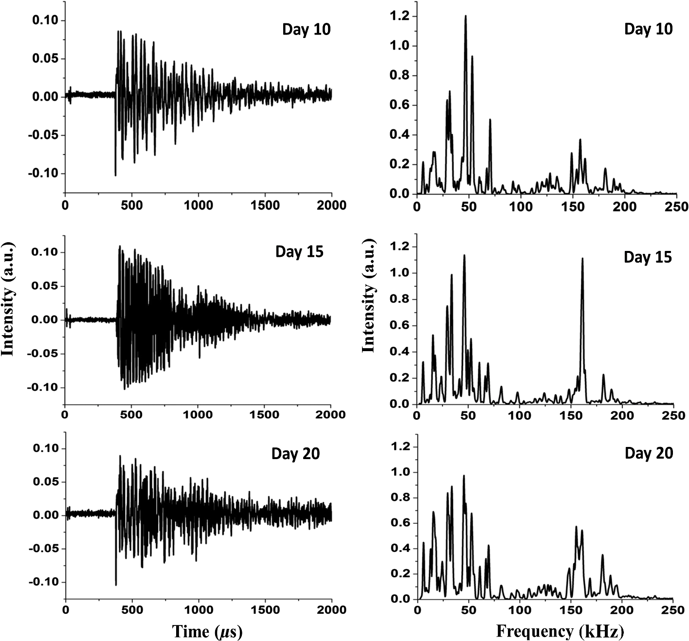

Initially, we looked into the frequency patterns of the samples belonging to D10, D15, and D20, and a gradual increase in the strength of certain frequencies 29.37, 29.69, and 30 kHz was observed with the progression of the tumor growth as shown in Fig. 4. The increase of frequency strengths was also found to be significant between D10 and D20 groups. However, no significant difference in the frequency strengths for D10 and D15 as well as D15 and D20 was observed. Although there were significant differences in the strengths of some other frequencies (33.75, 34.06, and 50 kHz) observed for D10 and D15 as well as D15 and D20, no specific trend was noticed in the variation. Hence, we found this region of 14 to 80 kHz had a high potential for inherent information, which may contribute to grouping the time points under study.

Fig. 4

Tumor growth assessment on some selected frequencies of days 10, 15, and 20 post MCF-7 cell line inoculation ($\text{mean}\pm \text{sem}$ indicated).

It is an established fact that the low-frequency components always travel faster through a medium. It can be correlated with the tumor growth/development observed in the present study in the case of low-frequency (0 to 30 kHz) components of the PA spectra discussed above. Further, there are reports in the literature^62–64 showing desmoplastic reactions in the stroma of neoplastic tissues in breast cancer conditions, resulting in overdeposition of dense fibrous tissues (mainly collagen I, III, and IV) and other extracellular matrix components. This leads to the formation of the solid lump within the tissue providing it with tensile strength, stiffness, and tightness. The acoustic waves in the present study are produced due to the absorption of 281 nm excitation by the tryptophan moieties of proteins in the tumor, which subsequently propagate through the tumor mass. Once the tumor tissue becomes stiffer and the free space gets filled, it facilitates the movement of the acoustic waves in a faster manner. This may be one of the reasons for the gradual increase observed in the strengths of the low-frequency (0 to 30 kHz) peaks in the present study. The irregularities in the peak intensity behavior above 30 kHz may be attributed to the inhomogeneity of the acoustic field in the tumor mass.⁶⁵ Also, in cancer cells, it has been observed that the cellular and the nuclear morphology differ from a normal cell. The major noticeable characteristic of the nuclei of cancer cells is that they are abnormally enlarged and have a folded shape.^66–68 Though a direct relationship is still not established between the nuclear morphology and the cancer phenotype, the nuclear changes in the cancer cells may be tumor type and stage specific.⁶⁷ Further, it has been noticed that even though the absorption maxima of DNA is at 260 nm, for proteins at 280 nm, the ratio of absorption coefficient for DNA to proteins is much less at 280 nm.^65–68 Thus, the low optical contrast between DNA and protein absorption at 281 nm might have contributed to the inhomogeneity of the acoustic field and affected the signal propagation.

In order to accomplish the discrimination among different time point groups under study, the corresponding PA FFT patterns were subjected to Haar and Morlet wavelet analysis one after the other, and the Morlet wavelet coefficients so obtained were used for extracting features for further analysis. As mentioned above, there were seven spectral features (mean, median, area under the curve, variance, standard deviation, skewness, and kurtosis) extracted, and using them, a feature matix of dimensions $216\text{spectra}\times 7\text{features}$ was prepared. This feature matrix was used for PCA and the first three PCs showing the maximum variance in the data that were selected. The percentage variance of PC1, PC2, and PC3 scores for day 10, day 15, and day 20 groups were found to be 87.40, 12.58, 0.009; 97.54, 2.44, 0.006; and 99.33, 0.65, 0.001%, respectively. From the above information, it is clear that the first two PC scores for all the three groups were sufficient to represent the maximum variability within the respective group of samples. Further, a comparison of log PC1 and log PC2 score values for the three groups by the Kruskal-Wallis test also revealed a significant difference among them. PC1 captured the maximum variability among the three groups ($p<0.0001$ ***). Dunn’s multiple comparison test has also shown a significant ($p<0.0001$ ***) difference with PC1 for D10 versus D15, D10 versus D20, and D15 versus D20, respectively. PC2 was also found to be significant ($p=0.0009$, ***), and Dunn’s multiple comparison test with PC2 for D10 versus D15 and D10 versus D20 was found to be significant. Hence, the subsequent logistic regression analysis was conducted using the logs of PC1 and PC2 scores only.

Once the first two PC components were found to contribute the maximum variance in the data as well as significance in their classification, the logs of PC1 and PC2 scores for 20 samples of all three groups under study were randomly chosen to form a calibration set and were used for making an appropriate decision boundary in the logistic regression with 100% specificity and sensitivity, respectively. Subsequently, log PC1 and PC2 scores of the remaining 52 samples in each group were tested against the calibration set decision boundary and the corresponding sensitivity, specificity, and accuracy of the classification was calculated. The correct prediction accuracy of the classification as well as the sample membership association with a particular group for D10 versus D15 was found to be 90.38 and 94.23%, respectively, with an overall accuracy of 92.31% as shown in Fig. 5(a). In the case of D15 versus D20, the correct prediction accuracy as well as the sample membership association to a particular group was 80.77 and 94.23%, respectively, along with overall accuracy of 87.5% for the analysis as shown in Fig. 5(b). The prediction accuracy and the membership association for D10 versus D20 analysis was found to be 92.31 and 98.08%, respectively, along with the overall accuracy of 95.2% as shown in Fig. 5(c). The prediction accuracy of the multiple comparision analysis performed with all three calibration sets taken together, making a decision boundary for each and testing the remaining samples of each group against the respective decision boundaries was found to be 90.38, 73.08, and 94.23% for D10 versus D15, D15 versus D20, and D10 versus D20, respectively [Fig. 5(d)]. The overall accuracy of the multiple comparison analysis was found to be 85.9% as shown in Fig. 5(d). The observed misclassifications in D15 versus D20 comparison may be due to the tumor heterogeneity during the growth period and the physiology of the cancer cells. Further, there are reports showing morphological changes within the developing tumors and their microenvironment influencing the light propagation and hence the acoustic velocity through them affecting the corresponding spectral characteristics.^47,48,65

Fig. 5

Discrimination of the photoacoustic spectra of tumor tissues of days 10, 15, and 20 for the spectral region 14.375 to 80.625 kHz by wavelet principal component analysis based logistic regression analysis: (a) day 10 versus 15, (b) day 15 versus 20, (c) day 10 versus 20, and (d) day 10 versus 15 versus 20, respectively.

In order to test the reproducibility of the discrimination models for D10 versus D15, D15 versus D20, and D10 versus D20 analysis, the receiver operator characteristics (ROC) curves for the same were also plotted as shown in Fig. 6. The area under the curves (AUC) for the ROC plots of D10 versus D15, D15 versus D20, and D10 versus D20 analysis were found to be 0.95, 0.85, and 0.93, respectively. These observations clearly demonstrate that the ROC-AUC values are approaching 1, indicating the potentiality of the analysis to show the significant discrimination among the different groups ($p<0.0001$) under study, suggesting the clinical implication of the analysis.

Fig. 6

The receiver operator characteristics plot of the discrimination analysis for day 10 versus 15, day 15 versus 20, and day 10 versus 20, respectively.

5.

Conclusion

The PA spectroscopy used to monitor the breast tumor development in the present study has clearly demonstrated its ability to capture the minor biochemical changes upon tumor development. The wavelet-PCA based logistic regression analysis, applied for the assessment of the tumor growth, has distinctly identified the unique spectral patterns in each group of the samples under study and accordingly differentiated the tumor progression. The sensitivity of the technique in capturing the minor biochemical changes along with the accuracy of identifying the tumor progression by using wavelet-PCA based logistic regression analysis has evidently provided its possible clinical implications. However, for identifying specific biomarkers of tumor progression and drawing a correlation with the early detection of the disease, further in-depth PA studies are warranted.