1.

Introduction

In recent years, optical molecular imaging (OMI) and related optical technique–based multimodality fusion methods have experienced notable growth and attracted considerable attention for their excellent temporal resolution, simple operation, and high cost-effectiveness. Furthermore, OMI has already been used for early stage cancer diagnosis, drug discovery, and disease treatment with the help of exogenous agents that provide detectable signals or endogenous molecules with optical signatures.^1–7 In particular, the application of OMI in vivo studies has greatly advanced our understanding of biology and medicine. Fluorescence molecular tomography (FMT) is one of the various modalities of OMI which has attracted considerable attention due to its high sensitivity and low cost, aiming at noninvasive and quantitative imaging of the biodistribution of fluorophores in deep tissues by upgrading the two-dimensional (2-D) fluorescence imaging to three-dimensional (3-D) in vivo detection.^8–10

Among FMT methods, it is well known that photon propagation models in biological tissues and inverse problems are the two main challenges, which have a marked effect on tomographic imaging performance.^11,12 To perform quantitative FMT, the forward photon propagation model needs to be solved, which can generate a linear system linking the internal unknown fluorescent source and the boundary measurements. Then, the fluorescent source distribution is reconstructed by solving the inverse problem. Currently, different reconstruction techniques for FMT have been proposed based on numerical techniques,^13,14 including the finite-difference method (FDM),¹⁵ finite-element method (FEM),¹⁶ and boundary element method (BEM).¹⁷ Among these methods, the FEM has become the most commonly used technique in FMT for its versatility, which makes it easily executable in complex heterogeneous geometrics.¹⁸ In particular, the acquired sparsity positive-definite FEM yields great numerical stability and efficiency, which has significantly contributed to the development of reconstruction algorithms.^19–22 However, FEM relies on strictly designed meshes connected together by nodes in a properly predefined manner. It has limitations including time consumption in mesh generation, difficulty in the case of adaptive analysis, and significant discretization error in extremely complicated geometry (such as bones).²³

In order to overcome the difficulty of 3-D meshing, the meshless method (MM) was recently proposed.²⁴ This technique uses only a set of nodes to represent the problem domain and its boundary. Without any point connectivity or element information, the burdensome mesh discretization is avoided, resulting in improved accuracy due to the decrease in the discretization error. It has been successfully applied to solve problems in solid mechanics, heat transfer, fluid flow, and so on.²⁵ Qin et al. have introduced MM in bioluminescence tomography (BLT)²² based on the Galerkin method. This work has shown a huge potential of MM in the field of optical imaging. Compared with the Galerkin-based methods, the compactly supported radial basis functions (CSRBFs) method possesses advantages in the following aspects: (1) it is a truly mesh-free algorithm; (2) it is space dimension independent in the sense that the order of convergence is $O(h^{d+1})$, where $h$ is the density of the collocation points and $d$ is the spatial dimension; and (3) in the context of scattered data interpolation, CSRBFs have spectral convergence orders.

In this paper, we introduce a meshless method for the reconstruction of FMT (MM-FMT) based on CSRBF, in order to improve the accuracy and efficiency of the reconstruction. The image domain is represented by a series of CSRBFs based on a direct collocation method, which guarantees the accuracy of the forward model of FMT. After formulating the inverse problem of MM-FMT based on the forward model, three different conventional algorithms, including Tikhonov regularization, L1-norm iteration shrinkage (IS),²⁶ and sparsity adaptive matching pursuit (SAMP),²⁷ are utilized to solve the inverse problem. Heterogeneous mouse model experiments and in vivo experiments are performed to validate the proposed method. We compare our results with those obtained by the FEM-based reconstruction methods (FEM-FMT). Results show that the proposed MM-FMT can achieve better performance.

This paper is organized as follows. Section 2 describes the details of the forward model of FMT and the proposed MM-FMT. Section 3 shows the results of numerical heterogeneous mouse experiments and in vivo experiments. Finally, Section 4 discusses the results and draws the conclusion.

2.

Method

2.3.

Direct Collocation with Compactly Supported Radial Basis Functions

For the reconstruction of FMT, we adopt CSRBFs to represent the image domain based on a direct collocation method to guarantee the accuracy. Figure 1 shows the schematic diagram of the method. First, we distribute the CSRBFs uniformly along the boundary of the image domain. The CSRBFs should be distributed densely to ensure the integrity and accuracy of the boundary. Then we randomly distribute the CSRBFs within the image domain, and the maximal distance between the adjacent centers of CSRBFs is set to be the compactly supported radius, which can avoid the leakage space inside the image domain.

Fig. 1

Direct collocation based on compactly supported radial basis functions (CSRBFs) and the schematic diagram of a CSRBF. (a) The boundary of the image domain is represented by a series of CSRBFs, which are uniformly distributed on the boundary. The red solid circle denotes the boundary of the image domain, and the black dots denote the centers of CSRBFs. The green-dashed circles represent the support regions of each CSRBF. (b) After the boundary discretization, the image domain is represented by randomly distributed CSRBFs. (c) The schematic diagram of a CSRBF.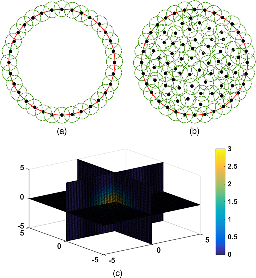

After the representation, the fluorescent distribution $X$ at node $r$ can be collocated by the CSRBFs as follows:

Eq. (8)

$$X(P,U)=\sum _{i=1}^L{\mu }_i{p}_i[d(r)]=PU,$$

where $P=[p_1,p_2,\dots ,p_L]$ is the matrix of CSRBFs, $U={[{\mu }_1,{\mu }_2,\dots ,{\mu }_L]}^T$ is the fluorescent intensity coefficient of the CSRBFs, and $L$ is the number of CSRBFs. Substituting Eq. (8) into Eq. (3), the inverse problem of FMT leads to a meshless formulation:

Eq. (9)

$$\begin{gathered} \underset{U}{\min }E(U)=\arg \underset{U\ge 0}{\min }\frac{1}{2}{\Vert APU-\mathrm{\Phi }\Vert }_2^2 \\ =\arg \underset{U\ge 0}{\min }\frac{1}{2}{\Vert TU-\mathrm{\Phi }\Vert }_2^2, \end{gathered}$$

where $T=AP$ is the meshless system matrix for FMT.

2.4.

Meshless Inverse Problem

Due to the multiple scatterings of photon propagation through heterogeneous biological tissues, the inverse problem of FMT is often highly ill-posed and ill-conditioned.^20,35 Although more fluorescence information can be captured by multiple spatial patterns of illumination, the problem may still be strongly ill-posed because of the sensitivity to noise and errors caused in the data-gathering process and raw data discretization.¹⁹ To obtain a reasonable solution, penalty terms are typically introduced to the objective function, which is considered as a priori information:

Eq. (10)

$$\underset{U}{\min }E(U)=\arg \underset{U\ge 0}{\min }\frac{1}{2}{\Vert TU-\mathrm{\Phi }\Vert }_2^2+\lambda R(U),$$

where $R(U)$ is the penalty function and $\lambda$ is a positive real number called the regularization parameter used to balance the two terms. Here, we consider the case when $R(U)$ is ${\Vert U\Vert }_P^p$ with $p=1,2$. In this case, the inverse problem with general Lp-norm regularization can be modified into

Eq. (11)

$$\underset{U}{\min }E(U)=\arg \underset{U\ge 0}{\min }\frac{1}{2}{\Vert TU-\mathrm{\Phi }\Vert }_2^2+\lambda {\Vert U\Vert }_p^p.$$

To get the optimal solution of Eq. (11), we adopt three different conventional algorithms, namely, Tikhonov regularization (where $p=2$), IS, and SAMP (where $p=1$), as described in the previous sections.

The procedure of the proposed MM-FMT is summarized in Fig. 2.

Fig. 2

Procedure of the proposed meshless reconstruction method for fluorescence molecular tomography (FMT) based on CSRBFs.

3.

Experiment and Results

In this section, both numerical simulation studies and in vivo mouse studies have been designed to evaluate the accuracy, robustness, and efficiency of the proposed method. All of the computational processing was completed on a personal computer with a 3.20 GHz Intel Core i5 CPU and 4 GB RAM.

To validate the performance of the reconstruction method, we utilize the position error (PE), the contrast-to-noise ratio (CNR), and computation time in this paper. The PE is defined to measure the accuracy of the results:

The CNR is also used in this paper as a metric to indicate whether the reconstructed object could be clearly distinguished from the background.³⁶ In this paper, we divide the image domain into two regions: volume of interest (VOI) and volume of background (VOB). VOI is defined according to the location and size of the reconstructed object, and VOB is the remaining part of the domain. CNR can be calculated by

3.1.

Results of the Heterogeneous Mouse Model

To generate the heterogeneous mouse model, an adult nude mouse was used to acquire the original dataset by micro-CT. All animals used in this study were purchased from the Laboratory Animal Center, Peking University, China, and followed the experimental protocol guidelines according to the Institutional Animal Care and Use Committee (IACUC) at Peking University (Permit Number: 2011-0039). In our study, it is supposed that there were two small tumors on the surface of the animal’s liver, which were the fluorescent targets to be detected. Only the torso section of the mouse was selected as the region to be investigated, as shown in Fig. 3(a). The diameters of the tumors were both set to 2 mm. The edge-to-edge distance of the two tumors was 9 mm. The major organs and tissues (heart, lungs, liver, kidneys, and muscle) were used to construct the heterogeneous mouse model, where the corresponding optical properties were assigned according to Table 2.³⁷ The excitation light sources were modeled as isotropic point sources located in the plane with a light intensity of 0.02 w. The measurements were taken with a 160 deg field of view, as shown in Fig. 3(b). In the experiments, a 5% Gaussian noise was added to the measurements to simulate the situation where practical fluorescence measurements were taken using a charge-coupled device (CCD) camera. Fluorescent images in a 360 deg full view were collected at every 45 deg, with eight projections adopted in total.

Table 2

Optical parameters of the mouse organs (units of μa and μs′: mm−1).

Tissue	μax	μsx′	μam	μsm′
Muscle	0.0052	1.08	0.0068	1.03
Heart	0.0083	1.01	0.0104	0.99
Lungs	0.0133	1.97	0.0203	1.95
Liver	0.0329	0.70	0.0176	0.65
Kidneys	0.0660	2.25	0.0380	2.02

Fig. 3

Image of the heterogeneous mouse model. (a) Three-dimensional (3-D) visualization of the model. (b) Cross-sectional image of the model in the plane $z=25\mathrm{mm}$, which contains the fluorophore. The white dots denote the location of the excitation light sources. T1 and T2 are two the tumors on the surface of the liver, which are the targets to be reconstructed.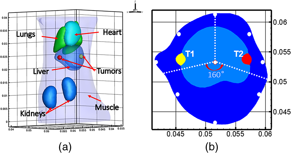

3.1.1.

Evaluation of reconstruction reliability

To verify the reconstruction reliability of the MM-FMT, we have conducted 50 reconstructions with different numbers of CSRBFs, denoted by the number of functions (NOFs). The NOFs can have a considerable effect on the reconstruction accuracy of MM-FMT when representing the image domain. In this section, the NOF was selected with different orders of magnitude, ranging from 100 to 5500. The reconstructions were performed using IS. The regularization parameters were both set to $1.0\times {10}^{-3}$, and the maximum iteration number was set to 200. The reconstruction results are partly delineated in Fig. 4, and the quantitative analysis is listed in Fig. 5.

Fig. 4

3-D views of the reconstructed results by meshless method FMT (MM-FMT) with different number of functions (NOFs). NOF was selected with different orders of magnitude, ranging from 100 to 5500. The red balls inside the image domain denote the real position of the tumors.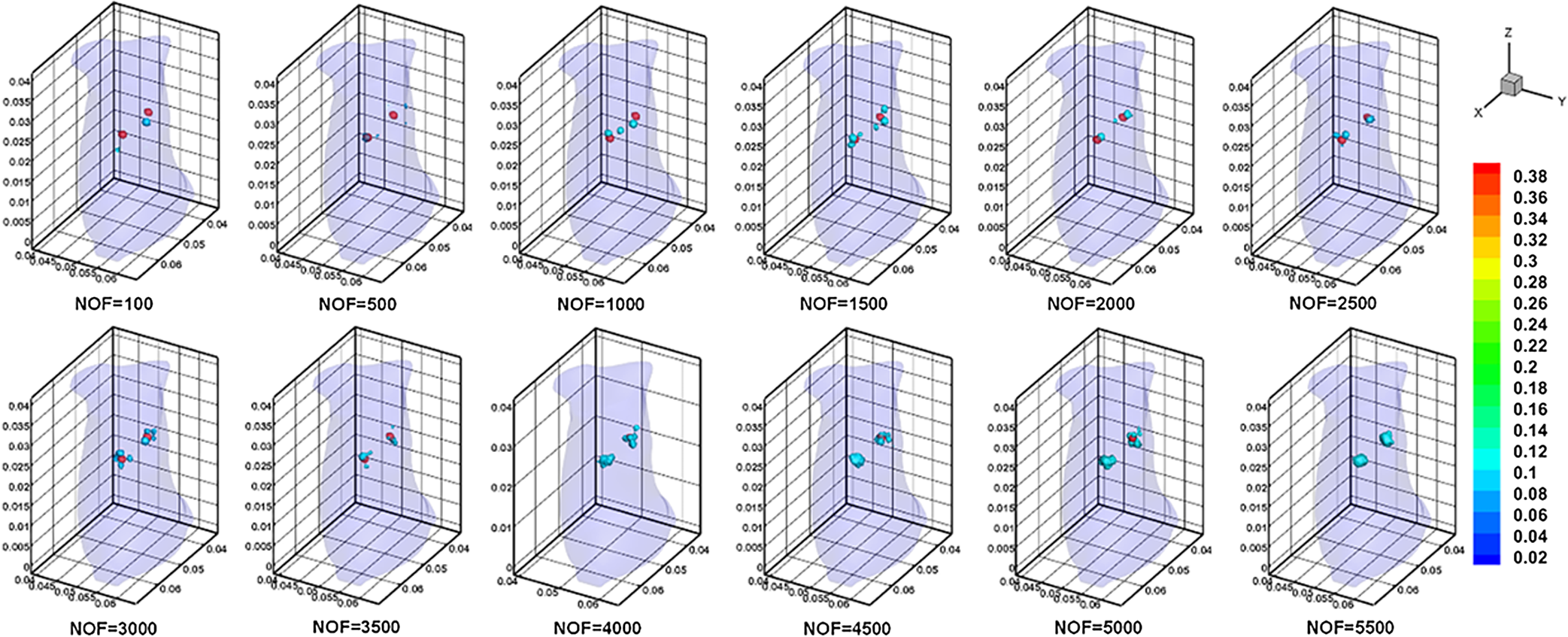

Fig. 5

Influence of NOF on position error (PE), contrast-to-noise ratio (CNR), and computation time in the numerical heterogeneous mouse experiments. (a) Chart of PE for two tumors with an increase in CNR. (b) Chart of CNR and computation time with the increase of CNR. The PE, CNR, and computation time were obtained according to the table below the chart, with the range of NOF from 100 to 5500.

From Fig. 5, we know that when the NOF is too small ($\mathrm{NOF}<=1000$), meaning the image domain is too sparsely discretized, the two fluorescent sources cannot be reconstructed at the same time, in which case the accuracy of reconstruction is not ensured either. As NOF increases, the accuracy of the reconstruction increases. However, a certain number of artifacts were found in the results when $\mathrm{NOF}>1000$, since the ill-posedness of the inverse problem increases as the NOF increases. This leads to a decrease in CNR and an increase in computation time. Because the CSRBFs are randomly distributed in the interior of the image domain, the reconstructions are not stable when $\mathrm{NOF}<=2500$. When $\mathrm{NOF}>2500$, the variation of the results begins to decrease, and the reconstruction tends to be stable. As can be concluded from the above results, the reconstruction results are satisfying when $\mathrm{NOF}>1500$. The reconstruction becomes stable when $\mathrm{NOF}>2500$.

3.1.2.

Evaluation of reconstruction efficiency

To examine the efficiency of the MM-FMT, we tested it using the numerical heterogeneous mouse model. In this section, we used both MM-FMT and FEM-FMT methods to reconstruct the internal tumors, where Tikhonov, IS, and SAMP were performed to more sufficiently illustrate the efficiency of the MM-FMT. For the FEM-FMT, we discretized the heterogeneous mouse model into 5624 nodes and 29,306 elements. For the purpose of comparison, we set $\mathrm{NOF}=5624$, which is equal to the number of nodes. The regularization parameters were both set to $1.0\times {10}^{-3}$, and the maximum iteration number was set to 200.

The reconstruction results for both MM-FMT and FEM-FMT via Tikhonov, IS, and SAMP are shown in Figs. 6 and 7, where Fig. 6 is the 3-D view and Fig. 7 is the cross-sectional view. The quantitative analysis of the two methods is listed in Table 3, where we include PE, CNR, and computation time. As seen in Figs. 6 and 7, both MM-FMT and FEM-FMT can achieve the reconstruction of the two tumors, except for the FEM-FMT via SAMP. The results of the MM-FMT are more condensed with smoother surfaces. The reconstruction regions of the MM-FMT are more accurate with smaller intensity variations, as can be seen from the PE and CNR values. Due to the same dimension of the reconstruction data, the computation times of the MM-FMT and FEM-FMT via the three algorithms have the same order of magnitude. In addition, the computation time of the center distribution of the MM-FMT (17.82 s) is much shorter than that of the mesh generation of the FEM-FMT (295.74 s). This can be attributed to the fact that the MM-FMT does not require the connective information of each center, so there is essentially no other additional operation for mesh generation, simplifying, smoothing, and filtering.

Table 3

Quantitative analysis of the meshless method fluorescence molecular tomography (MM-FMT) and finite-element method FMT (FEM-FMT) with three different methods.

Methods		PE(mm)		CNR	Time(s)
		T1	T2
MM-FMT	Tikhonov	0.45	0.59	10.6	336.44
	IS	0.38	0.36	16.9	65.26
	SAMP	1.02	0.71	30.7	22.02
FEM-FMT	Tikhonov	0.68	0.63	14.1	355.11
	IS	1.74	0.89	44.5	69.99
	SAMP	1.43	—	76.3	25.21

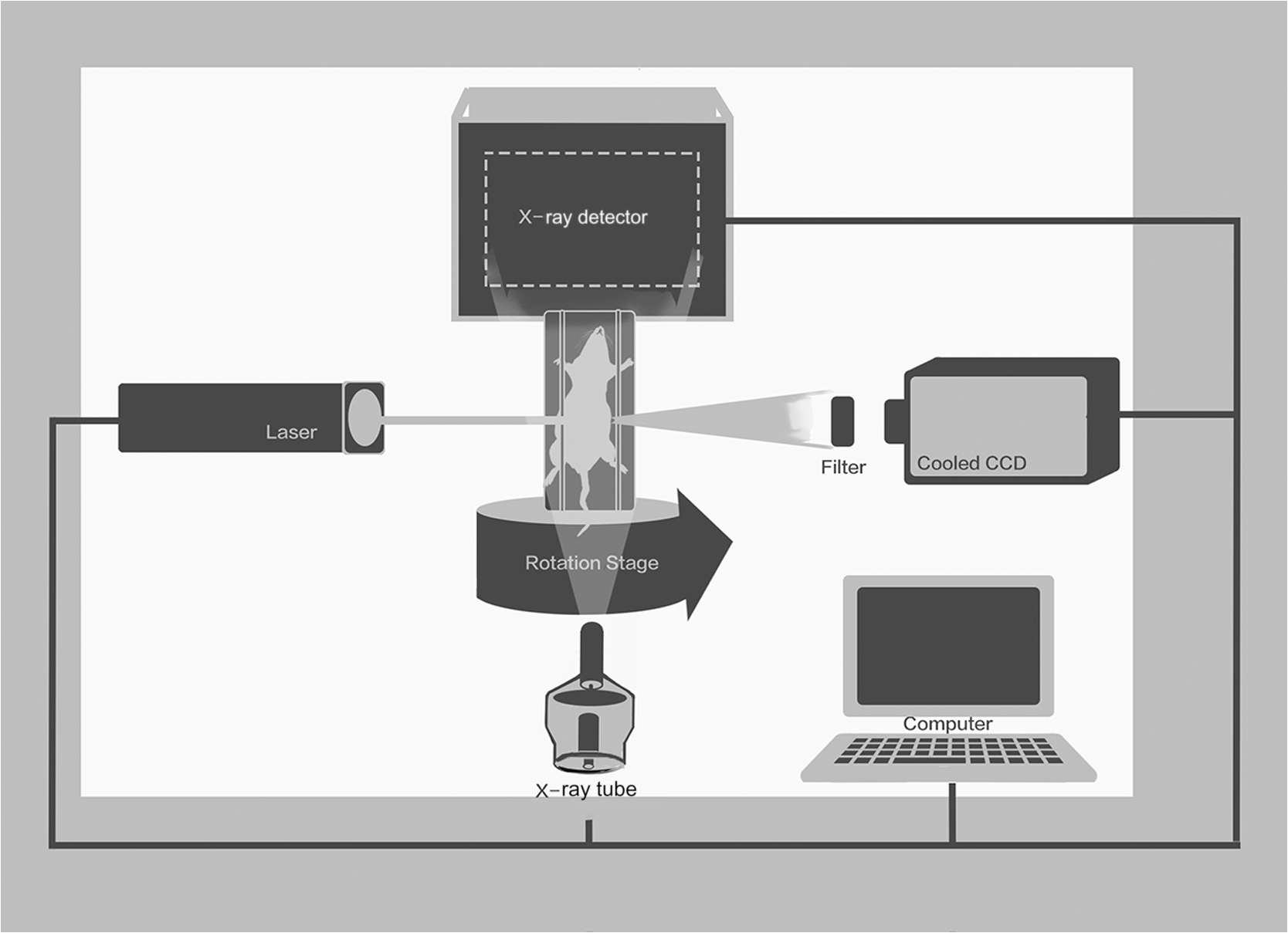
Fig. 6

3-D view of the reconstructed results of the heterogeneous mouse model with MM-FMT and FEM-FMT, using Tikhonov, IS, and sparsity adaptive matching pursuit (SAMP) methods. The first row lists the results of the MM-FMT, and the second row lists the results of the FEM-FMT. The columns denote the results obtained by Tikhonov, IS, and SAMP. The iso-surfaces in the figure denote the reconstruction results of the tumors. The threshold for the iso-surfaces is 30% of the maximum intensity. The red balls inside the image domain denote the real positions of the tumors.

Fig. 7

Cross-sectional view of the reconstructed results heterogeneous mouse model with MM-FMT and FEM-FMT. The first row lists the results of the MM-FMT, and the second row lists the results of the FEM-FMT. The columns denote the results obtained by Tikhonov, IS, and SAMP. The red circles mark the real positions of the tumors.

3.2.

Results of the In Vivo Experiment

To validate MM-FMT in a practical application, an in vivo mouse experiment on an adult Kunming mouse was conducted. For imaging purposes, the multimodality imaging system developed by our group^38–40 was used to acquire the experimental datasets, which is an integrative platform combining fluorescence imaging with micro-CT. For micro-CT scanning, the cone-beam x-ray generator (Oxford Instruments, 90 kV UltraBright Micro-focus Source) was operated in a continuous mode with a 55 kVp tube voltage, where 360 deg projections were scanned and the signal was accepted by an x-ray detector (Hamamatsu Photonics, C7943CA-02 Flat Panel Sensor). An ultrasensitive cooled CCD camera (Princeton Instruments, PIXIS: 1024) was used to obtain the multiview fluorescent images. The excitation light was generated by a 671-nm continuous wave (CW) laser. The schematic diagram of the multimodality imaging system is shown in Fig. 8. We collected the fluorescence measurements in transillumination mode.

Fig. 8

Schematic diagram of the hybrid FMT/XCT system.

A plastic fluorescent bead was implanted inside the hypogastrium of the mouse, which was filled with a cy5.5 solution with a concentration of 2000 nM. This fluorescent solution has a peak excitation wavelength of 671 nm with quantum efficiency of 0.23, and the emission wavelength is 710 nm.⁴¹ After imaging, the micro-CT volume and fluorescent images were acquired by the dual-modality system. In order to build the heterogeneous mouse mode, the micro-CT volume was segmented into several parts⁴⁰ (muscle, heart, lungs, liver, kidneys, and bones), as shown in Fig. 9. The corresponding optical properties were assigned to different organs and tissues according to Table 4.⁴² Then the fluorescent images were mapped onto the 3-D micro-CT volume via a 3-D surface flux reconstruction algorithm,⁴³ so the photon distribution of the fluorescent signals on the mouse surface was obtained, which was indispensable for reconstruction.

Table 4

Optical parameters of the mouse organs at 670 and 710 nm (units of μa and μs′: mm−1).

Materials	670 nm		710 nm
	μax	μsx′	μam	μsm′
Muscle	0.0849	0.4273	0.0563	0.3792
Heart	0.0574	0.9620	0.383	0.9050
Lungs	0.1918	2.1720	0.1266	2.1240
Liver	0.3437	0.6770	0.2283	0.6480
Kidneys	0.0644	2.2480	0.0430	2.1090
Bones	0.0593	2.4900	0.0393	2.3400

Fig. 9

Anatomical structure of the mouse. (a) Transverse view. (b) Sagittal view. (c) Coronal view. The yellow square marker in (a–c) illustrates the location of the fluorescent bead. (d) 3-D visualization of the mouse. The red dot in the graph corresponds to the fluorescent source.

After finishing the above procedure, the MM-FMT and FEM-FMT were both performed on the mouse through three different algorithms (Tikhonov, IS, and SAMP). The image domain of the mouse was discretized into 5639 nodes and 33,627 elements for FEM-FMT and 5639 CSRBFs for MM-FMT. The 3-D reconstruction results of MM-FMT and FEM-FMT are shown in Fig. 10. The cross-sectional views are given in Fig. 11. In addition, the quantitative analysis of the reconstruction results is listed in Table 5.

Table 5

Quantitative analysis of the in vivo experiment with MM-and FEM-FMT.

Methods		PE(mm)	CNR	Time(s)
MM-FMT	Tikhonov	0.93	17.9	275.66
	IS	1.82	120.7	59.16
	SAMP	0.44	62.6	43.64
FEM-FMT	Tikhonov	—	10.5	271.38
	IS	2.56	113.7	54.93
	SAMP	0.98	76.5	44.48

Fig. 10

3-D view of the reconstruction results for the in vivo experiment with MM-FMT and FEM-FMT, via Tikhonov, IS, and SAMP.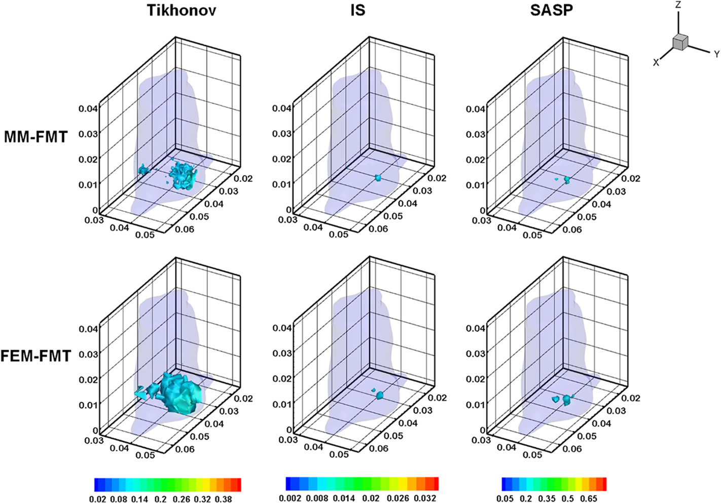

Fig. 11

Cross-sectional views of the reconstruction results of in vivo experiment with MM-FMT and FEM-FMT, via Tikhonov, IS, and SAMP. The first row lists the results of MM-FMT, and the second row lists the results of FEM-FMT. The third row lists the standard CT cross-sectional slices, which involve the fluorescent source. The columns denote the results obtained by Tikhonov, IS, and SAMP. The black square markers denote the actual location of the fluorescent source.

Similar to the numerical heterogeneous mouse experiments, better reconstruction results are achieved by the MM-FMT. The CT scan could determine the location of the internal fluorescent bead, since the bead was wrapped in a plastic material (Fig. 11). Compared with the real location of the fluorescent bead, the MM-FMT does not perform as well as in numerical studies, but the reconstruction accuracy is still acceptable. Quantitative analysis of the performance further demonstrates the superiority of the MM-FMT.

4.

Discussion and Conclusion

FMT has been rapidly developed in recent years for its advantages in the study of physiological and pathological processes in vivo at cellular and molecular levels. Research of the inverse problem of FMT is critical as the solution to the inverse problem, which is central to the accuracy and efficiency of the reconstruction. However, the application scope of the existing analytical and statistical techniques is currently limited by the different weaknesses inherent in each method. Developing more powerful numerical techniques is needed for better applicability and higher efficiency of FMT, particularly in the case of more complicated geometrics. In this paper, we presented a CSRBF-based meshless method to solve the inverse problem in heterogeneous biological tissues. Compared with the conventional FEM analysis, the MM-FMT can obtain better reconstruction performance.

It has been shown in Section 3.1.1 that the NOF is serious for the reconstruction. When the NOF is small, the computation cost is reduced, but the accuracy is undesirable. When the NOF increases, the computation cost and the accuracy both increase. When $\mathrm{NOF}>2500$, the reconstruction results obtained by the MM-FMT demonstrate good performance (Figs. 4 and 5). In this paper, we chose the larger NOF to ensure accuracy. In future work, we will do some research to find the optimal NOF for the application of FMT.

Compared with FEM-FMT, better accuracy can be obtained with MM-FMT (Figs. 6 and 7 and Table 3). This is due to the fact that the meshless method can express the image domain continuously, avoiding the discretization error as in FEM to a certain degree. Besides, the reconstruction results of the in vivo experiment validate the feasibility of MM-FMT in a practical application.

In this paper, the MM-FMT was performed via three conventional methods including Tikhonov, IS, and SAMP. More effective reconstruction methods for FMT can be combined with MM-FMT to achieve better performance. In this paper, we distributed the center of CSRBFs with direct collocation. The adaptive collocation method can be further evaluated to more accurately and effectively express the image domain.

In conclusion, we have presented a meshless reconstruction based on CSRBFs to increase the accuracy of FMT. By choosing an appropriate number of CSRBFs to discretize the image domain, the image to be constructed can be more accurately expressed, thus avoiding the limitations of conventional FEM. The results of the numerical heterogeneous mouse experiments and in vivo experiment demonstrate the superiority of the MM-FMT.