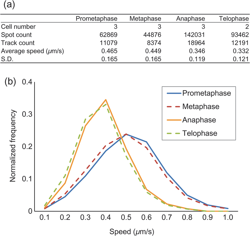
1.

Introduction

The nature of the actuating mechanism that drives the mitotic apparatus remains an important unresolved question despite extensive investigation in this field spanning more than a century. The concept of a mitotic apparatus was originally based on microscopy studies performed in the late 1800s.^1,2 In early studies, images of cells and subcellular organelles were produced from fixed specimens. Such fixatives often introduced artifacts and consequently the existence of macromolecular structures within cells remained controversial. The first observation of a spindle apparatus within a living cell was made using polarizing light microscopy by Schmidt and Inoué.^3–5 Inoué⁵ built an improved polarizing microscope that could image weakly birefringent materials and demonstrated for the first time the filamentous nature of the mitotic spindle within living cells using time-lapse imaging. Subsequently, Inoué and Sato et al.^6,7 demonstrated that microtubules were the sole constituent of spindle fibers and established a basis for understanding how microtubule dynamics generate the forces for chromosome movement.

The discovery and practical application of green fluorescent protein (GFP) by Shimomura⁸ and Chalfie⁹ as well as the development of color variations by Tsien^10,11 has revolutionized the field of live imaging, by enabling the engineering and expression of chimeric fluorescent proteins in target cells (reviewed in Ref. 12). Microtubules are 25-nm diameter tubular polymers composed of two proteins, $\alpha$- and $\beta$-tubulin. GFP-fused tubulin can be incorporated into microtubules without disrupting their function in many cell types, allowing the visualization of both cytoplasmic and spindle microtubules.^13,14 In in vitro studies using purified proteins, microtubules exhibit repeated stochastic growth and shortening, a behavior referred to as “dynamic instability.”^15,16 Visualization of microtubule behavior in living cells with GFP-tubulin or microinjected fluorescently labeled tubulin has proven that dynamic instability is a general property of microtubules and is fundamental in generating various cellular microtubule network patterns (reviewed in Refs. 1718.19.–20). However, owing to the performance limitations of fluorescence microscopes, the detection of discrete filaments has been limited to thinner regions of the cell, such as flattened membranous lamellipodia, or the imaging of small organisms such as yeasts, which only contain a few microtubule filaments. Although imaging methods such as poleward flux detection using photoactivatable fluorescent probes²¹ and fluorescent speckle microscopy²² have enabled the indirect observation of microtubule dynamics within the mitotic spindle, the direct observation of all the individual filaments within the spindle apparatus has never been achieved.

We have previously generated a GFP fusion of the EB1 protein (EB1-GFP), which localizes to microtubule plus-ends [Fig. 1(a)],^23,24 and demonstrated its utility as an analytical tool for the study of microtubule dynamics.^25,26 Live-cell imaging revealed that EB1-GFP binds selectively to the growing ends of microtubules, forming a comet shape with a short axis diameter of approximately 25 nm and an anteroposteriorly elongated tail of up to 500 nm.^23,25,27 EB1 functions as a hub, tethering microtubule ends to various subcellular structures generating an asymmetric filament network.^17,28–30 Fluorescently tagged EB1 family proteins, including both EB1 and EB3, faithfully mark the growing portions of microtubules, even within the dense microtubule networks of the cell interior such as those found in columnar-shaped epithelial cells²⁵ and neuronal filaments.³¹ Time-lapse imaging and tracking of EB1-GFP comets allows the generation of microtubule growth trajectories and the measurement of growth speed.³² However, until recently, image acquisition and analysis has been predominantly limited to a two-dimensional (2-D) plane, because the spatiotemporal resolution of conventional fluorescence microscopes is insufficient to follow the three-dimensional (3-D) motion of EB1-GFP comets that can move at several hundreds of nanometers per second.

Fig. 1

(a) Distribution of EB1-GFP in a mitotic HeLa cell at metaphase. HeLa cells (clone A1) stably expressing EB1-GFP (green) and H2B-TagRFP (magenta) were fixed and immunostained with an anti-$\alpha$-tubulin antibody (red) to enable the position of microtubule ends to be identified. Images were collected with a LSM780 laser scanning confocal microscope. Examples of EB1-GFP comets at the ends of astral microtubules are indicated with arrowheads. Scale bar: $5\mu \mathrm{m}$. (b) An example of a lattice light-sheet (LLS) microscope image. The image was imported into Imaris 8 software and displayed in three-dimensional (3-D) space. The image was rotated horizontally about 90° from one direction (left) to another (right). At both angles, discrete EB1-GFP comets were visible at the tips of astral microtubules growing radially toward the cell cortex and within the spindle apparatus. Scale bars: $5\mu \mathrm{m}$. See also Video 1 (QuickTime, 8 MB) [URL: http://dx.doi.org/10.1117/1.JBO.20.10.101206.1].

Recently, we succeeded in the 3-D tracking of EB1-GFP movement throughout the cell cytoplasm using the recently developed lattice light-sheet (LLS) microscope, which enables 3-D scanning at subsecond intervals with high-spatial resolution.³³ This technology is an advanced type of light-sheet microscopy, which uses a separate excitation lens perpendicular to the wide-field detection lens to confine the illumination to the focal plane.^34,35 In contrast to the conventional light sheet created with several-micron-thick Gaussian beams, the lattice light sheet is generated from a massive parallel array of nondiffracting light beams that mutually interfere to create an ultrathin light sheet extending over cellular dimensions.^33,36 Spreading the excitation light across many foci greatly reduces the intensity at any single focus, and in turn, reduces fluorescence photobleaching and phototoxicity. This strategy allowed us to image whole cells for hundreds of volumes at subsecond intervals.

LLS technology generates thousands of numerical data sets containing far more information than can be practically analyzed using conventional approaches. Therefore, automated computational strategies are required to extract biologically significant information in an efficient and reproducible manner. To analyze the 3-D motion of particles, automated object tracking methods by digital image processing have been developed and their application in biology is becoming popular.^32,37 However, many challenges still exist regarding the interpretation of 3-D data. These challenges include the classification, selection, or grouping of objects of interest and the geometric presentation and interpretation of volumetric data. To this end, computational 3-D geometry and geometric modeling techniques are also necessary. In addition, the analysis of biological image data, which may be very noisy and is often multidimensional, requires improvement. Morita et al.³⁸ established a computing system for the processing and visualization of large numbers of 3-D images, which can be offered through cloud-based platforms. Combining this system with mathematical computational techniques, we analyzed 3-D time-lapse images of EB1-GFP obtained with LLS microscopy to gain new insights into microtubule dynamics.

Our analysis enabled both the microtubule growth speed and direction to be identified within the mitotic spindle apparatuses in 3-D. These observations support recent hypotheses emphasizing the important contribution of noncentrosomal microtubules, which cannot be detected using conventional light microscopy techniques, in spindle organization and chromosome segregation. The observations presented in this study push the limits of conventional microscopic analysis and demonstrate the power of this analysis framework, which we believe will be applicable and of benefit in a wide range of research fields.

2.

Image Acquisition and Processing

2.2.

Image Visualization

Images were imported into Imaris 8 software (Bitplane, South Windsor, Connecticut). LLS microscopy provides a high-definition 3-D image that can be observed from any angle with similar resolving power,³³ which is largely beyond the capabilities of conventional laser confocal fluorescence microscopes, enabling the discrimination of detailed structures in 3-D space within cells. Importantly, individual EB1-GFP comets were detectable even deep within the mitotic spindle apparatus [Fig. 1(b); Video 1], which is in sharp contrast to conventional confocal images in which the spindle structure appears as a single fluorescent mass [Fig. 1(a)].

LLS microscopy also provided a detailed view of the interaction of microtubule ends with the cell cortex. When an image of an anaphase cell was rotated and observed from the side, many EB1-GFP comets reaching the cell cortex were detected [Fig. 2; Videos 2 and 3]. In particular, at the basal cortex where the cell was attached to the substratum, EB1-GFP comets often ran along the plane of the surface [Fig. 2(c), arrowheads], which was in contrast to other regions, where the majority of EB1-GFP comets disappeared shortly after reaching the cortex [Fig. 2(b), arrows]. These observations suggest the nonuniform regulation of microtubule activity within different cortical regions of the cell. Observation of the detailed behavior of fine structures inside cells and the overall picture concurrently is a major advance in the whole-cell imaging by LLS microscopy because previously we were only able to observe cellular components from a fixed angle [optical axis direction ($z$)] and in a limited area (due to the limitation of imaging speed) in live imaging.

Fig. 2

Observation of interactions between EB1-GFP comets and the cell cortex. (a) Side view of an anaphase cell. The plane of the coverslip ($xy$ direction) is indicated. (b) Superimposition of EB1-GFP trajectories generated by automated 3-D comet tracking. Arrows indicate trajectories that disappeared shortly after reaching the cortex. (c) Enlarged time-lapse images of the boxed area in (b). Some trajectories run along the basal cell cortex (white and yellow arrowheads). Time is shown in s:ms. Scale bars: $5\mu \mathrm{m}$ (b), $2\mu \mathrm{m}$ (c). Color bar: time (s:ms). See also Video 2 (QuickTime, 5.1 MB) and Video 3 (QuickTime, 9.9 MB). [URL: http://dx.doi.org/10.1117/1.JBO.20.10.101206.2]. [URL: http://dx.doi.org/10.1117/1.JBO.20.10.101206.3].

2.3.

Image Preprocessing for Quantitative Analysis

For the quantitative and statistical analysis of microtubule growth, especially inside spindles, we tried automated 3-D tracking of EB1-GFP comet movements throughout the cell using only single-channel images for GFP that were collected using the fastest acquisition mode. Subsequent analysis of EB1-GFP trajectory data in 3-D space enabled the quantification of microtubule growth within the cell. All images used were collected at 0.755-s intervals over a 56.625-s duration (75 frames) at different mitotic phases after nuclear membrane breakdown, i.e., during prometaphase, metaphase, anaphase, and telophase [for typical mitotic figures, see Fig. 5(a)]. Detailed procedures for image processing are described in the Appendix.

2.3.1.

Drift correction of spindle position

We performed several steps of image preprocessing to facilitate the high-precision tracking of EB1-GFP comets. First, we corrected for the movement of spindles. The spindle apparatus can serve as a useful frame of reference during cell division; however, it often rotates and changes orientation during division, which can reduce the accuracy of the positional measurements obtained for each EB1-GFP comet and can make interpretation of the results difficult. Consequently, in order to compare all datasets under a common reference frame, changes in the angular orientation of the spindle were compensated for using a drift correction method. The positions of the two centrosomes were automatically tracked and their displacements then used to correct for orientational and rotational drift for the whole data set using the Correct Drift function in Imaris software. As shown in Fig. 3(a) and Video 4, drift correction reduced changes in the positions of the spindle and chromosomes.

Fig. 3

Effects of drift correction. (a) Time-lapse images of a HeLa cell (clone A1) acquired with an LLS microscope (1.510-s interval, 50 frames) were imported into Imaris 8 software and displayed in 3-D space. The first frame is shown on the left. The middle and right panels show the maximum intensity projection (MIP) of all 50 frames. The spindle apparatus can often rotate in any direction in cells as shown in the middle panel. This rotational drift was corrected for by using the positions of the two centrosomes as a reference (right). Scale bar: $5\mu \mathrm{m}$. See also Video 4 (QuickTime, 8.2 MB) [URL: http://dx.doi.org/10.1117/1.JBO.20.10.101206.4]. (b) Sum Slice projection (SSP) images generated from 30 frames of a metaphase cell before and after drift correction. After the drift correction, spots estimated to be kinetochore-associated EB1-GFP signals (arrowheads) and bundle of trajectories toward the kinetochores became visible. (c) Enlarged MIP images of astral EB1-GFP. MIP images of two-increment 11th to 31th time-lapse images (10 frames) of a metaphase cell before and after drift correction to observe the shape of an individual comet. The shape change of each comet was not evident, but the image was somewhat blurred after correction. (d) Comparison of EB1-GFP intensity profiles. The line profiles of two EB1-GFP comets ($0.53\text{-}\mu \mathrm{m}$ width, shown in the left panels) were obtained and plotted in the right panel. The results are shown as relative intensity (right top) and normalized intensity standardized to the peak intensity (right bottom). The peak intensity was reduced by approximately 10% while the full width at half maximum of normalized intensity was increased by approximately 10% after drift correction. Scale bars: $5\mu \mathrm{m}$ (a), (b), $3\mu \mathrm{m}$ (c), (d). All the above images were created by capturing the Imaris screen view presenting objects in 3-D space.

After drift correction, the repetitive appearance of EB1-GFP along the same trajectories toward kinetochores aided the visualization of the paths of growth of kinetochore microtubules in the Sum Slice projection (SSP) image [Fig. 3(b), arrows] and spots adjacent to the kinetochores [Fig. 3(b), arrowheads], which were observed in PtK1 cells.⁴² These observations indicate that fast 3-D scanning of mitotic HeLa cells by LLS microscopy faithfully captures common mitotic processes in a smaller cell type.

In the drift corrected images, the change in shape of each EB1-GFP comet was not evident, but the images were blurred [Fig. 3(c)]. Therefore, we compared intensity profiles of isolated EB1-GFP comets and found that the peak intensity was reduced by approximately 10% while the full width at half maximum of normalized intensity was increased by approximately 10% in the drift corrected image [Fig. 3(d)], although we were not able to know what kind of method Imaris software applied. This may affect the EB1-GFP comet detection capability, especially for small, low-intensity comets. Nonetheless, we used the drift correction procedure because quantification of microtubule behavior (growth angle and position of EB1-GFP trajectories) is the main purpose of this study. It should be also noted that in the drift corrected images, information regarding the relative position of microtubule ends and cell cortex could not be retained.

2.3.2.

Intensity equalization and signal enhancement

We performed two-step image quality improvement processing of the drift-corrected data to compensate for the effects of channel bleed-through and photobleaching. Only the signal from the green (EB1-GFP) channel from the dual-labeled HeLa cells was required for automated tracking. However, bleed-through from the red channel [Fig. 4(a)] as well as the time-dependent photo-bleaching of the signal in the green channel [Fig. 4(c)] were apparent from the analysis of image data. To reduce these unfavorable effects, images were subjected to both (1) intensity equalization and (2) small target enhancement by top-hat transformation, using VCAT5 software.³⁸ (1) For intensity equalization, the intensity of a 3-D image at each time point was normalized using the average intensity value for the whole $xyz$ volume [Fig. 4(c)]. (2) To enhance EB1-GFP comet signals, we employed a top-hat transformation, an image processing technique for extracting small elements from images with a variable background.⁴³ In acquired images, the area occupied by a single EB1-GFP comet ranged from $3\times 3\text{pixels}$ in the case of a small comet to $7\times 10\text{pixels}$ for the largest comets. We used opening radius $R=2.0\text{pixels}$ in the $xy$ plane and $R=1.0\text{pixel}$ in the $z$ direction taking into account the 3-D voxel pitch ($0.100\times 0.100\times 0.217\mu {\mathrm{m}}^3$), and its effect is shown in Figs. 4(a) and 4(b); Videos 5 and 6.

Fig. 4

Effects of image preprocessing. After intensity equalization, the images were processed for image enhancement by top-hat transformation (opening radius $R=2.0\text{pixels}$ in the $xy$ plane and $R=1.0\text{pixel}$ because the voxel pitch is $0.100\times 0.100\times 0.217\mu {\mathrm{m}}^3$). An example of the resulting image (a) and a line profile [3 pixel line width, indicated with yellow lines in (a)] of signal intensity (b) are shown. Arrowheads in (a) indicate the bleed-through from the red channel labeling chromosomes. (c) Effect of intensity equalization and top-hat transformation on the 3-D volume intensity. Examples of a metaphase cell and a telophase cell are shown. Average intensities of 3-D volume at each time point before and after preprocessing are plotted. See also Videos 5 (QuickTime 3.3 MB) and 6 (QuickTime 3.1 MB) [URL: http://dx.doi.org/10.1117/1.JBO.20.10.101206.5]. [URL: http://dx.doi.org/10.1117/1.JBO.20.10.101206.6].

2.4.

Automated tracking of EB1-GFP movement

The preprocessed images were imported into Imaris 8 software. EB1-GFP comets were automatically detected by local contrast mode and automated tracking was subsequently executed using the Autoregressive Motion algorithm, which predicts that the spot will move again the same distance and in the same direction. To eliminate possible tracking errors, several filter algorithms, including Max speed, track duration and straightness, were applied based on the assumption that microtubule growth is essentially straight with a variable, but limited elongation rate. We needed to adjust the parameters in different mitotic phases (for detailed procedures, see Appendix).

Examples of the resultant trajectories are shown in Fig. 5(b) and Videos 7–12. Several cells in different mitotic phases [Fig. 5(a)] were analyzed, and a statistical summary of the distribution of microtubule track speeds for each phase are shown in Fig. 6. Consistent with our original observation using conventional 2-D timelapse imaging²³ and previous observation by LLS microscopy, in which EB1-GFP comet speed was measured using different software,³³ the population of fast-growing microtubules grew toward the prometaphase and metaphase where it peaked, then decreased gradually toward the telophase.

Fig. 5

Automated tracking of EB1-GFP comets. (a) Typical patterns of microtubule and chromosome organization at each indicated mitotic phase. HeLa cells (clone A1) were fixed and immunostained for microtubules and examined by confocal microscopy. Microtubule and histone H2B-TagRFP are shown in white and red, respectively. (b) Representative images of EB1-GFP trajectories in HeLa cells (clone A1) at different mitotic phases. The trajectories were generated by automated tracking. Results from the first 40 frames of a corrected 75-frame sequence are shown with a color code designating the moving speed. The color bar indicates the speed range for the instantaneous speed of EB1-GFP comets (0.3 to $0.6\mu \mathrm{m}/\mathrm{s}$). See also Videos 7–12 [QuickTime, 7.1 MB (7); 7.0 MB (8); 7.7 MB (9); 7.5 MB (10); 7.7 MB (11), 7.4 MB (12)] [URL: http://dx.doi.org/10.1117/1.JBO.20.10.101206.7]. [URL: http://dx.doi.org/10.1117/1.JBO.20.10.101206.8]. [URL: http://dx.doi.org/10.1117/1.JBO.20.10.101206.9]. [URL: http://dx.doi.org/10.1117/1.JBO.20.10.101206.10]. [URL: http://dx.doi.org/10.1117/1.JBO.20.10.101206.11]. [URL: http://dx.doi.org/10.1117/1.JBO.20.10.101206.12]. Scale bars: $5\mu \mathrm{m}$.

Fig. 6

(a) Statistical summary of EB1-GFP comet speed data for each mitotic phase obtained by averaging data obtained from several cells. (b) Frequency distribution of comet speeds.

2.5.

Analysis of Spatial Variations in Microtubule Dynamics

The dynamic and spatial properties of EB1-GFP trajectories were further analyzed by mathematical computing techniques and the calculated results were geometrically represented in 3-D space by developing a pipeline implemented in MATLAB^® R2012a software (The Mathwork Inc., Natick, Massachusetts).

2.5.1.

Classification of trajectories by growth speed

First, mean travel speeds were grouped into $0.1\text{-}\mu \mathrm{m}/\mathrm{s}$ intervals bins and displayed separately for each range [Fig. 7]. The trend showed a good correlation with the distribution of movement speeds plotted in Fig. 6, in which the high-speed population was largest in prometaphase and metaphase, with mean speeds decreasing toward telophase. An interesting feature that this presentation method highlights is the trend for trajectories with fast or slow migration speeds to be associated with particular regions of the cell. Fast trajectories often originated near the centrosomes, while slowly migrating ones tended to accumulate at the intercentrosome region, considering the slowly moving EB1-GFP comet traveling along microtubules associating with kinetochores. Because spindle microtubules exhibit poleward flux caused by their depolymerization at the minus ends,²¹ it is reasonable that a net movement of the comet is underestimated in the kinetochore fibers. In addition, it is possible that separation of the centrosome during anaphase/telophase affects measurement of the comet speed. In the data used, variations in the centrosome separation distance were less than $1\mu \mathrm{m}$ during the observation period (56.625 s) (data not shown). Therefore, its effects are likely to be negligible.

Fig. 7

Subcellular distribution of EB1-GFP comet trajectories moving at different rates in each mitotic phase. Comet speed data were divided into 10 classes spanning the entire data range (0 to $1\mu \mathrm{m}/\mathrm{s}$). Data included in the 0.2 to $0.7\mu \mathrm{m}/\mathrm{s}$ range are shown. Each bin contains data equal to or more than the first threshold and less than the second threshold. Blue and red triangles indicate centrosomes. Color bar indicates the mean speed ($\mu \mathrm{m}/\mathrm{s}$). Cyan and yellow-green dots indicate the start and end position of trajectories, respectively. In this figure, trajectories initiated in the 1st to 30th frames are displayed.

2.5.2.

Analysis of growth angle and location of trajectories

We also measured the angle between the direction of EB1-GFP movement and the centrosomal axis [defined as the straight line between the two centrosomes; Fig. 8(a)]. The results for each cell are shown separately in this figure. The data clearly show that the distribution of growth trajectory angles was similar for cells in the same mitotic phase, while the overall distribution patterns were different among the different mitotic phases. The random orientation of trajectories observed in prometaphase shifted to a directional pattern, which was estimated to associate with the formation of spindle fibers or the spindle midzone at later stages. In the case of the prometaphase cells #2 and #3, a population of trajectories having shallower angles to the centrosomal axis started increasing, indicating that this cell was on the transition stage from prometaphase to metaphase. From an experimental validation perspective, these observations demonstrate the reproducibility achieved by our detection and automatic tracking.

Fig. 8

(a) Illustration of the method used to analyze the distribution of EB1-GFP trajectories in 3-D space. Spheres centered at centrosomes (red and blue triangles) and with radii equal to the intercentrosomal distance were generated and then divided into 10 spherical zones of equal radial length (top). The centrosomal axis is indicated with a blue line (bottom). The angle between each EB1-GFP comet trajectory and the centrosomal axis (yellow) was calculated. (b) The distribution of EB1-GFP comet trajectory angles was plotted according to their distance from the centrosome. The direction of the $x$-axis (centrosomal axis) of one of the centrosomes was inverted by 180 deg and superimposed on another centrosome position to represent data from both centrosomes in a single coordinate. Each bin contains data equal to or more than the first threshold and less than the second threshold. The results from three different cells (two in the case of telophase) were plotted in line plots and histograms.

Next, we arranged EB1-GFP trajectories according to their subcellular location at prometaphase, metaphase, and anaphase (Fig. 9). Each EB1-GFP trajectory was assigned to one of 10 data bins according to the radial distance of its start position from the centrosome. The EB1-GFP trajectories of different data bins were then presented separately [Fig. 9(a)]. It can clearly be seen that many trajectories began their growth at positions located away from the centrosomes, an observation that is inconsistent with the established notion that the centrosome is the main microtubule nucleating structure. Notably, in the anaphase cell, large numbers of trajectories were aligned parallel with one another at the midpoint between the two centrosomes and most of their start points resided in zones 4 and 5 (an area between the centrosome and the midzone). It is possible that many of these were generated by regrowth from existing microtubules, and not by de novo nucleation, but that the gradual positional shift in the start points as mitosis progressed is clear [Figs. 9(b) and 9(c)], suggesting nucleation of microtubules at the noncentrosomal sites.

Fig. 9

(a) Trajectories of EB1-GFP comets grouped according to the position of the first track point are displayed separately for each indicated spherical zone [see Fig. 8(a)]. Representative results for cells in prometaphase, metaphase, and late anaphase are shown. Orange and cyan dots indicate start and end positions, respectively. The color bar indicates the mean speed ($\mu \mathrm{m}/\mathrm{s}$). The distribution of the start and end point positions of trajectories in cells shown in (a) are plotted according to their start position in the line graph in (b) and the histogram in (c). Each bin contains data equal to or more than the first threshold and less than the second threshold.

The EB1-GFP imaging alone cannot distinguish de novo nucleation from regrowth of existing microtubules, because it visualizes only the growing phase of microtubule dynamic instability. Therefore, to examine the above possibility further, we analyzed the angle of EB1-GFP comet movement relative to the centrosomal axis in vertical zones dividing the intercentrosomal space. If the angle of comet movement deviates from a line projected from the centrosome toward the comet position, this indicates that the microtubule is unlikely to have initiated from that centrosome (because microtubule outgrowth is essentially straight). Results shown in Fig. 10 indicate that a subpopulation of microtubules grew at an off-axis orientation, and support the possibility of noncentrosomal microtubule nucleation.

Fig. 10

(a) Illustration of the method used to analyze the distribution of EB1-GFP trajectories in 3-D space. The 3-D space was divided vertically and cylindrically about the centrosomal axis into 70 bins. The vertical zones and the cylindrical divisions were numbered as shown in (b). (c) In the green zone around the origin, trajectories initiated from the centrosome can take on any angle (green arrows). However, if the trajectory angle between EB1-GFP movement and the centrosomal axis is larger than 45 deg (red arrow) in the yellow-colored area, these microtubules are unlikely to originate from the centrosomes based on an assumption that microtubules grow in a straight line. (d) Representative results for cells in prometaphase, metaphase, anaphase, late anaphase, and telophase are shown in line plots grouped by division. Each bin contains data equal to or more than the first threshold and less than the second threshold.

Recently a new model for interpolar microtubule assembly that is dependent upon augmin, a protein complex implicated in the nucleation of noncentrosomal microtubules, was proposed.⁴⁴ In this model, a subset of microtubules in early anaphase is generated de novo around chromosomes in the interzone to generate central spindle microtubules that ensure completion of cytokinesis.⁴⁴ Observations made in our study are consistent with this hypothesis. As this example shows, our study clearly demonstrates the applicability of our analytical strategy to a wide range of research areas that require precise 3-D information to understand more comprehensively the processes driving the actions of cellular machinery at the whole-cell level.

3.

Summary and Outlook

After more than 20 years since the discovery and practical application of GFP, the recent development of LLS microscopy now enables live whole-cell imaging in 3-D with high-spatial resolution and subsecond acquisition rates. On one hand, this technological advance greatly increases the potential of GFP as a subcellular fluorescent reporter, because it enables the movements of individual fluorescent proteins to be monitored throughout an entire cell with high spatiotemporal resolution. On the other hand, the enormous volume of multidimensional data provided by LLS microscopy represents a significant challenge because it contains complex information that cannot be analyzed using conventional methods that are mostly designed for 2-D platforms and often require substantial user interaction. Therefore, the introduction of computational techniques supporting automatic detection and geometric modeling is essential for interpreting these data.

In this study, we imaged the motion of EB1-GFP in live mitotic HeLa cells to obtain 3-D trajectories of microtubule growth within the spindle apparatus using an LLS microscope. Image processing prior to automated tracking and mathematical computing allowed us to identify microtubule growth trajectories with different dynamic properties and to map their coordinates in 3-D space. As expected, the reconstructed 3-D displays revealed many microtubules started growing from regions near centrosomes and subsequently extended radially outward. These microtubules are also observable with conventional microscopes and are known as astral microtubules. However, an important observation was the existence of another group of microtubules that grew from a point distant from the centrosome.

It has long been considered that centrosomes are the main microtubule nucleation sites. However, a pioneering in vitro reconstitution study⁴⁵ and recent studies^44–47 revealed that the centrosome itself is not critical for bipolar spindle formation and spindle microtubules can also be generated by noncentrosomal pathways; i.e., the chromatin-dependent pathway and the spindle microtubule-based microtubule generation mediated by augmin. These hypotheses were strongly supported by a later report describing the continued development of early mouse embryos in the absence of mature centrosomes until the 64-cell stage (early blastocyst).⁴⁸ Studies such as this demonstrate that biological knowledge acquired through observations made with conventional microscopy techniques may overlook an unknown number of important phenomena. Therefore, as new technologies become available, we should extensively re-examine not only mitosis, but a variety of other fundamental biological processes, including cellular morphogenesis and polarization, differentiated/undifferentiated processes, and membrane/organelle trafficking, at spatiotemporal resolutions that permit a more detailed analysis of the molecular machinery of living cells.

Our methods described here combined LLS microscopy with image processing and mathematical computing techniques, and our results demonstrated the great potential of this approach. However, before its application in the analysis of other novel molecular mechanisms, we need to improve our automated tracking and image processing techniques. Most importantly for our purpose, improved accuracy of EB1-GFP comet detection is critical. In the case of EB1-GFP detection, one effective way would be the expansion of a 2-D template matching method described by Matov et al.³² to 3-D space, using the average EB1-comet shape. In addition, because the automatic detection algorithm is sensitive to both specimen drift and variations in image intensity, methods that enable highly precise drift correction and image intensity equalization over time and in 3-D space are required for most applications. Changes in image intensity can be caused both by fluctuations in the excitation light intensity and by fluctuations in the distance of an object from the light source (i.e., depth within the specimen). Simple intensity equalization of a whole volume, such as that used in this study, is not sufficient for accurate and complete automatic detection. Indeed, some weak signals within the specimen that were furthermost from the light source or were most aberrated by the cell body were not detected by our analysis. We, therefore, need to develop a technique that can compensate for a three-dimensionally distributed intensity gradient within a specimen and optical heterogeneities within the specimen.

Another factor that requires improvement is microscopes. Faster acquisition will improve the accuracy of object tracking. Limiting the scanning area can speed up the frame rate by several factors. This will also be highly beneficial for multicolor imaging. To improve the detection of objects at deeper regions, an adaptive optics system, which corrects for the blurring effects of emitted light distorted in the specimen in real time, is expected to bring an important improvement.

In summary, once we have improved the computational analysis framework, its combined application with LLS microscopy will enable spatiotemporal information regarding the movements of fluorescent proteins within living specimens to be acquired with previously unobtainable precision. We, therefore, believe that this method of advanced imaging analysis will prove to be an invaluable research tool for a wide range of scientific fields in the future.