Self-referenced, microdegree, optical rotation polarimeter for biomedical applications: an analysis

Zeev Weissman; Doron Goldberg

doi:10.1117/1.JBO.21.7.071104

22 December 2015 Self-referenced, microdegree, optical rotation polarimeter for biomedical applications: an analysis

Zeev Weissman, Doron Goldberg

Author Affiliations +

Journal of Biomedical Optics, Vol. 21, Issue 7, 071104 (December 2015). https://doi.org/10.1117/1.JBO.21.7.071104

Abstract

We comprehensively analyze the performance of a type of optical rotation (OR) polarimeter, which has been designed from the outset to fit the special requirements of two major applications: general chiral detection during the separation of optical isomers by high-pressure liquid chromatography systems in the pharmaceutical industry, and monitoring of glucose in the interstitial fluid of diabetics by a fully implanted long-term optical sensor. Both very demanding applications call for an OR polarimeter that can be miniaturized while maintaining high resolution and accuracy in the microdegree range in the face of considerable noise from various sources. These two characteristics—miniature size and immunity to noise—set this polarimeter apart from the traditional OR polarimeters currently in use, which are both bulky and very susceptible to noise. The following detailed analysis demonstrates the advantages of this polarimeter and its potential as an analytic and diagnostic tool.

1. Introduction

Optical rotation (OR) polarimeters are valuable tools for measuring the concentration of optically active substances in a solution. Such polarimeters are used extensively in the food and pharmaceutical industries and also in research laboratories. High-end, very sensitive polarimeters can be found mainly in the pharmaceutical industry.¹ These sophisticated polarimeters are used for the detection of chiral molecules (a.k.a. optical isomers or enantiomers) as they are separated by high-pressure liquid chromatography (HPLC) systems during the process of drug manufacturing, where in many cases the complete separation of the active chiral isomer of a drug from its (sometimes toxic) counterpart is required by the U.S. Food and Drug Administration (FDA).²^,³

Similar high-end polarimeters have also been tried, so far unsuccessfully, for the noninvasive monitoring of glucose—mainly in the aqueous humor of the eye of diabetics.⁴ The strong scattering by the tissues and birefringence artifacts have prevented reliable noninvasive glucose measurements by a polarimeter.⁵ However, glucose at its physiological concentration in the interstitial fluid (ISF), a transparent fluid surrounding the cells in our body, has a relatively strong optical activity (OA). All other ISF metabolites, except for proteins, have negligible combined OA (our unpublished results). This situation offers a unique opportunity for the polarimetric detection of glucose by a fully implanted device. Therefore, it is possible that a miniature accurate polarimeter could be used as a future continuous glucose monitor (CGM) suitable for long-term implantation in diabetics, as has already been suggested in the past.⁶

The typical OR polarimeter currently in commercial use in the pharmaceutical industry is the Faraday rotation (FR) polarimeter.³ Such polarimeters are based on a principle first described by Gillham⁷ and successfully implemented by Yeung et al.,⁸ in which the angle of the linearly polarized light beam is constantly modulated by a Faraday rotator. This modulation results in a significant amplification, because the OA signal becomes proportional to the rotation angle, as opposed to its square in ordinary null polarimeters. Unfortunately, FR polarimeters have two fundamental limitations. The first limitation is their sensitivity to polarization noise—in particular refractive index (RI) artifacts, known as pseudorotation.⁹^,¹⁰ This essentially degrades their limit of detection (LOD) in actual operating situations. The second limitation is their size. Modern polarimeters are bulky (typically the size of a desktop PC¹¹) and expensive devices, which cannot be easily integrated with the existing equipment.

The same applies to another important type of OR polarimeters, the optical heterodyne (OH) polarimeter. The OH method facilitates signal amplification, which can thus provide higher sensitivity. In principle, OH polarimeters, first introduced by King et al.¹² and Mitsui and Sakurai,¹³ have a resolution comparable to that of FR polarimeters.¹³ However, their system is substantially complex, and, in addition, they should be just as sensitive to polarization noise as their older FR counterparts. Indeed, OH polarimeters described in the literature, although sensitive,¹⁴^–¹⁶ seem to be severely limited by such noise.¹⁴^–¹⁷

Intracavity OR polarimetry is a third, less explored method to measure OR with increased sensitivity.¹⁸^–²⁰ Bougas et al.¹⁸ have recently described a chiral cavity ring down (CCRD) polarimeter, which uses an intracavity modulated Faraday rotator to overcome the depolarizing effect of linear birefringence and translates optical rotation into a proportional frequency change. Their method seems to be less sensitive to polarization noise than FR and OH polarimetries. Furthermore, the authors expect a high-potential OA sensitivity, although currently it is still in the millidegree range. The complexity and size of the CCRD polarimeter seem substantial and may not be amenable to miniaturization.

The specifications required from an HPLC polarimetric detector are determined by the conditions encountered in the flow-cell of the HPLC system and the OA and concentration of the separated chiral molecules. The optically active molecules moving inside the tubing of the HPLC system form a plug with a Gaussian concentration profile, which consequently appears at the detector as a Gaussian-like rotation pulse. The baseline rotation level is usually influenced by artifacts and therefore is sometimes not zero. The pulse height [or more accurately, its area under the curve (AUC)] varies with the concentration. The LOD of the polarimeter is determined by its resolution and sensitivity to various sources of noise. The higher the resolution and immunity to noise, the lower the LOD. Lower LOD means better quality of drugs and efficiency of handling expensive reagents.

The requirements for a glucose monitoring polarimeter are determined by the physiological characteristics of the sugar. The concentration of blood glucose in healthy humans is 80 to $120 mg / dL$ . In diabetics, this concentration spans a much wider range of 50 to $400 mg / dL$ . The accuracy required by the 2013 ISO standard for blood glucose monitors is $\pm 15 mg / dL$ .²¹ For a polarimeter with a 10-mm optical path length, these values translate into ORs of 0.0038 to 0.0058, 0.0024 to 0.0192, and $\pm 0.00072 \deg$ , respectively. A fully implanted polarimeter capable of accurately and reliably measuring such ORs in the ISF could, in principle, be used for CGM in diabetics. When the polarimeter’s light beam is not blocked by strong scattering in the completely transparent ISF, the measurement of the sugar’s OA can prove superior, in both specificity and accuracy, to the measurement, e.g., of its near-infrared absorption spectrum. As a solid-state device, a polarimetry-based implanted CGM will have the potential to be sufficiently reliable in order to control an insulin pump in a closed-loop system termed artificial pancreas (AP)—a long-sought solution for diabetes still waiting for a suitable sensor.

We have recently described a type of high-resolution OR polarimeter,²² which we believe can overcome the shortcomings of similar FR and OH polarimeters. It uses a built-in reference mechanism that compensates for polarization noises, as well as a simple gain mechanism that contributes to LOD reduction. Furthermore, this optical configuration is amenable for miniaturization, possibly to the size of modern pacemakers.

Both applications described above create a substantial motivation to miniaturize the polarimeter. A miniaturized device with low LOD, immunity to polarization noises, and a reasonably stable operation—even under unstable environmental conditions—would have merit for both HPLC chiral detection and glucose monitoring. A small-footprint HPLC chiral detector, which also solves the pseudorotation problem currently plaguing commercial HPLC polarimeters, could more easily be integrated into existing HPLC equipment and gain wider acceptance in the pharmaceutical industry. Considerable miniaturization is certainly a prerequisite for an implanted polarimetry-based CGM in order to facilitate its implantation by a simple surgical procedure. We strongly believe that if this optical CGM can be realized, it will provide a reliable in vivo CGM suitable for AP operation—an issue that unfortunately has remained only partially solved to date.

However, miniaturization poses some challenges. One of them is the fact that some of the degrees of freedom available in an optical table model are absent in a miniaturized device, or are, at least, substantially more limited. For example, the rotational precision with which components can be positioned is more coarse than that available on an optical bench. Another issue is the quality of the optical components. Typically, for reasons of volume and cost, plate geometry is preferable for a miniaturized device. Nonetheless, the performance of plate components is typically lower (e.g., a plate polarizer would typically have a lower extinction ratio (ER) in comparison with birefringent polarizers). A third issue is the extent of the feasible miniaturization. For example, what is the shortest optical path length that can still provide the required optical performance?

Thus, to advance miniaturization, there is a need for a deeper quantitative understanding of the performance limits and limiting factors of this new type of polarimeter. This, essentially, is the purpose of the current article. It provides a detailed analysis of the polarimeter, as well as some of our more recent experimental results. The content of the article following this introductory section is arranged into five additional sections. Section 2 outlines the mathematical model based on the Jones calculus formalism.²³ Section 3 deals with the main aspects of performance of the polarimeter, including the angular LOD, linearity, dynamic range, and drift sensitivities, which are analyzed in detail. Section 4 contains an analysis of the susceptibility of the polarimeter to wavelength and temperature drifts. Section 5 is a discussion of the results of the previous sections, mainly from the perspective of future miniaturization of the polarimeter. Finally, Sec. 6 concludes the article.

2. Modeling the Polarimeter

2.1.

Polarimeter

The configuration of the polarimeter is illustrated in Fig. 1. The principle of operation was discussed in detail in our previous paper.²² In short, the measured optically active substance is moving through the flow-cell and slightly rotates the $E$ -field vector of a linearly polarized light beam propagating into the cell, perpendicularly to the direction of the flow. The beam then propagates through a variable electro-optic (EO) retarder that modulates (with a frequency of 10 to 50 Hz) the beam’s differential phase delay, between 0 and $π / 2$ radians. The beam is then reflected by a mirror and goes back into the variable retarder. At $0, π / 2$ retardance states, the same beam serves, alternately, as a reference and measurement beam, respectively. For each modulation period of the EO retarder, the measurement and reference photocurrents are subtracted. The difference between these two values is the differential photocurrent, which represents the optical rotation for the respective sampling moment.

Fig. 1

The optical configuration of the optical rotation (OR) polarimeter.

2.2.

Mathematical Model

To analyze the evolution of the polarization state as the beam traverses its optical path, we use the following Jones calculus:²³

Eq. (1)

(\begin{matrix} E_{x}^{\det} \\ E_{z}^{\det} \end{matrix}) = [An] \cdot [{BS}_{ref}] \cdot [{FC}_{in}] \cdot [{OA}_{left}] \cdot [{FC}_{out}] \cdot [{EO}_{1}] \cdot [Mirror] \cdot [{EO}_{2}] \cdot [{FC}_{out}] \cdot [{OA}_{right}] \cdot [{FC}_{in}] \cdot [{BS}_{pass}] \cdot [Pol] \cdot (\begin{matrix} E_{x}^{source} \\ E_{z}^{source} \end{matrix}),

where

E^{\det}

and

E^{source}

are the electric fields in the

\hat{x}

and

\hat{z}

directions [in accordance with the directions of our

x

-cut,

y

-propagating EO (RTP, Raicol Crystals Ltd., Israel) retarder, as described below]. The specific Jones matrices are given in Appendix A.

The photocurrent provided by the detector is given by

Eq. (2)

I_{PD} = \frac{{| E_{x}^{\det} |}^{2} + {| E_{z}^{\det} |}^{2}}{{| E_{x}^{source} |}^{2} + {| E_{z}^{source} |}^{2}} P_{source} \cdot T_{power}^{In \to Out} \cdot R_{λ} + i_{noise} \cdot randn,

where

T_{power}^{In \to Out}

accounts for the optical power loss incurred by the light beam as it propagates along the polarimeter (mostly due to diffraction and scattering),

R_{λ}

is the detector’s responsivity, and randn represents a random number generator with a normal distribution and unity standard deviation.

The noise current is

Eq. (3)

i_{noise} = \sqrt{i_{johnson}^{2} + i_{SD}^{2} + i_{SL}^{2}} .

The components of the noise current are the thermal (Johnson) noise and shot noises related to the dark and signal currents, respectively,

Eq. (4)

i_{johnson} = \sqrt{\frac{4 \cdot k_{B} \cdot {BW}_{n} \cdot T}{R_{sh}}}, i_{SD} = \sqrt{2 \cdot q_{e} \cdot {BW}_{n} \cdot I_{dark}}, i_{SL} = \sqrt{2 \cdot q_{e} \cdot {BW}_{n} \cdot R_{λ} P_{signal}},

where

Eq. (5)

P_{signal} = \frac{{| E_{x}^{\det} |}^{2} + {| E_{z}^{\det} |}^{2}}{{| E_{x}^{source} |}^{2} + {| E_{z}^{source} |}^{2}} P_{source} * T_{power}^{In \to Out} .

The relevant parameter values (as well as other specific data) are given in Appendix B.

2.3.

Component Positioning and Misalignments

The positioning of the optical components and the relevant angular parameters are described in Fig. 2.

Fig. 2

The positioning of the optical components and the angular parameters. PX, BX, and CX are the axial deviation angles with respect to the nominal (ideal) positioning. BR is the total amount of birefringence of the passive optical components. Note that the beam splitter and the flow-cell’s optical windows are assumed to have identical birefringence axis and deviation (BX). Also note that an optical gain is obtained by slightly rotating the polarizer (rather than the analyzer, which remains in its nominal position). This is unlike the original description in our previous publication.²²

In this figure, the analyzer position is used as reference. BX is the axial position of the birefringence of all the passive optical components, namely the optical windows and the beam splitter (the assignment of identical BX for all passive components was done for the sake of simplicity). CX is the angular deviation of the main axis of the EO crystal. Both BX and CX are unwanted, and an effort should be made to minimize them. In contrast, PX, the angular deviation of the polarizer with respect to its ideal (perpendicular) position, is less problematic. In fact, within a range of few degrees, such a deviation serves the purpose of increasing the OA signal, as discussed below.

3. Analysis—Performance

In Secs. 3 and 4, two types of aspects of the polarimeter are examined in detail: performance issues and susceptibility to temperature drifts.

The basic set of parameter values used throughout the following analysis is specified in Appendix B. For each of the subsections 3.1–3.6, the other relevant parameter values are indicated in the figures.

Throughout the analysis, the following numerical experiment is carried out: a Gaussian-like temporal rotation pulse is induced inside the flow-cell. In reality, this rotation pulse is caused by the entrance of a Gaussian-like plug of an optically active substance into the flow-cell. The resulting photocurrent is read at the signal photodiode as a function of time, and the differential photocurrent is subsequently calculated. An illustration of the relevant typical signals is shown in Fig. 3.

Fig. 3

The main signals of the OR polarimeter calculated throughout this article: (a) the Gaussian-like optical activity (OA) rotation pulse inside the flow-cell. (b) The voltage waveform on the RTP electro-optic (EO) retarder zoomed in to an interval of 0.6 s. (c) The resulting raw photocurrent at the signal detector. (d) The EO retardance resulting from applying the voltage shown in (b), with 0 and $π / 2$ single-pass retardances marked by circles and crosses, respectively. (e) The differential photocurrent calculated as the difference between the 0 and $π / 2$ raw sampled photocurrent vectors as marked in (f). (f) Zoom-in on the raw photocurrent waveform with 0 and $π / 2$ single-pass retardances marked by circles and crosses, respectively. In what follows, it is primarily the differential photocurrent that is referred to.

We start with performance analysis—specifically with a numerical demonstration of the two salient features of the polarimeter: a self-reference mechanism that eliminates non-OA artifact noises and a gain mechanism used here, which we previously²² termed tilted analyzer gain mechanism (TAGM). Because for practical reasons we now prefer to rotate the polarizer, we hereby rename it rotated polarizer gain mechanism (RPGM). This demonstration is followed by an analysis of some other performance aspects.

3.1.

Self-Reference Mechanism

This mechanism is mainly aimed at canceling out rotation artifacts that are not due to optical activity per se. Such artifacts are often called pseudorotation (PR) signals and are caused by RI gradients that may slightly tilt the light beam. The self-reference mechanism cancels the PR signal and leaves the OA signal intact. An example is given in Fig. 4. A pulse of PR slightly precedes a pulse of OA rotation, which is 10 times smaller [see Fig. 4(a)]. Without the self-reference, the measurement signal would look like Fig. 4(c). However, the reference signal, representing the net-PR component [see Fig. 4(d)], facilitates canceling this component out [see Fig. 4(e)].

Fig. 4

The main signals of the OR polarimeter calculated for a case in which a large pseudorotation (PR) signal artifact masks the OA signal: (a) the PR signal (dotted-blue line) and the OA (solid line) signals. (b) The raw photocurrent. (c) The measurement photocurrent. (d) The reference photocurrent. (e) The differential (net) photocurrent.

An example of the operation of the self-referencing system is shown in Fig. 5. We can see the large PR peak (caused in this case by pressure fluctuation induced by sample injection) that precedes the rotation pulse (marked by an arrow) and is more than one order of magnitude larger than the rotation pulse. Yet, by using the reference mechanism and the processing algorithm described above, this pseudopeak is nulled and the small OA peak is revealed in the net (differential photocurrent) signal.

Fig. 5

The operation of the self-referencing mechanism. The passage of the glucose sample ( $1 mg / dL$ ) in the flow-cell creates considerable noise as a result of changes in the refractive index. This PR noise affects (a) both the measurement and the reference signals and, therefore, can be easily subtracted, leaving only (b) the net signal (lower panel). The arrow marks a strong PR peak caused by pressure fluctuation during the injection of the sample.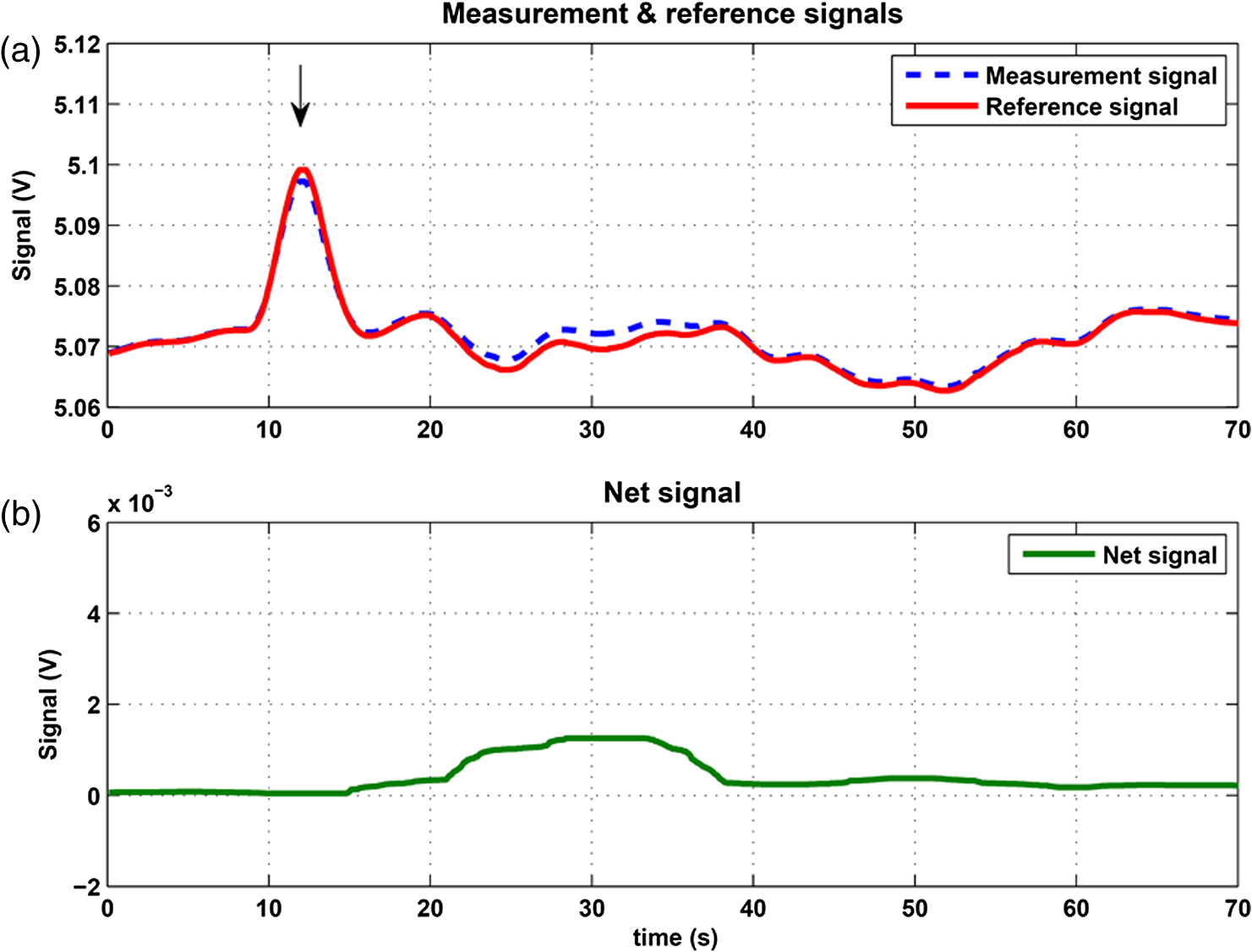

3.2.

Rotated Polarizer Gain Mechanism

Usually, the polarizer and the analyzer are perpendicular. However, this may not necessarily be the optimal position. In fact, by slightly deviating from this perpendicular position, i.e., by rotating the polarizer (or the analyzer, for that matter) by a small angular amount PX, one is able to increase the photocurrent sensitivity of the polarimeter relative to that obtained in the perfectly perpendicular position. In a sense, some optical “gain” of the angular signal is obtained this way. We have previously termed this TAGM,²¹ although we note that rotating the polarizer (instead of the analyzer) was found to be somewhat more effective in canceling small rotations, which result from RI PR artifacts.

The principle behind the RPGM mechanism is illustrated in Fig. 6.

Fig. 6

The principle of the rotated polarizer gain mechanism (RPGM). Rotating the polarizer by angle PX increases the OA-dependent photocurrent by a factor of 2 PX.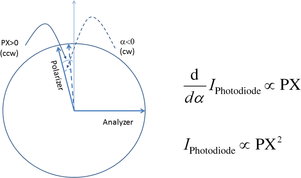

At the photodiode, by rotating the polarizer in Fig. 1 (labeled Pol), following the analyzer, the photocurrent is given by

Eq. (6)

I_{photodiode} \propto \sin^{2} (PX + α) \approx {PX}^{2} + 2 α \cdot PX + α^{2} \approx {PX}^{2} .

Because typically, PX, $α ≪ 1$ and $PX ≫ α$ . The derivative of this photocurrent (and consequently of the differential photocurrent) with respect to the OA rotation angle $α$ is

Eq. (7)

\frac{d}{d α} I_{photodiode} \propto 2 PX .

Thus, the changes in photocurrent and in the differential photocurrent are proportional to

{PX}^{2}

and PX, respectively. The effect of this mechanism on the photocurrent and differential photocurrent signals is illustrated in Fig. 7.

Fig. 7

The RPGM. (lower panels). The photocurrent and (upper panels) differential photocurrent increase in proportion to ${PX}^{2}$ and PX, respectively. For example, the difference between the plateau levels of (b) and (a) is about a quarter of the respective difference between (c) and (a). On the other hand, the difference between the pulse peaks of (e) and (d) is half the respective difference between (f) and (d). Note that in all subfigures, the rotation pulse is Gaussian, $20 μ \deg$ high, and the baseline rotation is zero.

Evidently, as the angle PX is increased, the differential photocurrent is increased proportionally. This very simple gain mechanism is essentially as efficient as that of OH polarimeters, but without the added complexity.²² However, note that in practice, the use of this mechanism is not without limits, as at some point the photodiode tends to saturate. In our polarimeter, saturation occurs at $PX \sim 2 \deg$ .

3.3.

Angular Limit of Detection

The angular LOD (or the resolution) of the polarimeter is defined as the smallest detectable incremental change of the rotation angle that is discernible in the differential photocurrent signal. It is defined as the smallest change that yields a signal-to-noise ratio (SNR) of 3. The result of a respective simulation is given in Fig. 8. It is based on the characteristics of a specific photodiode model (S 1226-18BQ, Hamamatsu, Japan), which is used throughout the calculation. This is a reasonably sensitive detector, although there are other more sensitive photodiodes that would probably yield a lower LOD.

Fig. 8

(a)–(d) The calculated differential photocurrent from which the angular limit of detection is inferred. It is calculated for two levels of the optical source power and two values of the rotation pulse. The thick dashed lines represent the running-average filtering (10 samples window) of the photocurrent signal. (e) Experimental differential photocurrent for $0.5 mg / dL$ glucose pulse in a 10 mm flow-cell equivalent to $\sim 23 μ \deg$ OA rotation pulse.

The signal is calculated for two rotation values and two source power levels, with and without smoothing, by means of a 10-point low-pass filter. Two parameters are calculated for each case: (1) the standard deviation of the noise $σ_{n}$ and (2) SNR, where the signal is defined as the Gaussian-like peak height, above the shoulders. The two parameters are inserted in each graph.

As can be expected, the differential photocurrent signal is less noisy as the source power increases, and consequently the LOD is lower. For example, for a 3-mW laser source [(c) and (d)] with low-pass filtering and using the above criteria ( $SNR = 3$ ), the LOD is $\sim 5 μ \deg$ , whereas for the 1-mW laser source [(a) and (b)], the LOD is $\sim 9 μ \deg$ . The implication is that by using a more powerful light source and a more sensitive photodiode, the shot-noise limit can be pushed down further.

For a comparison, (e) shows the results of a recent actual measurement. In this experiment, the laser power was 1 mW. In this case, for $SNR = 3$ , the LOD is $\sim 37 μ \deg$ .

By comparing the 1-mW source cases of (b) and (e) in Fig. 8, it appears that our current best experimental result exceeds the shot-noise LOD limit by a factor of $\sim 4$ . This difference seems to stem from two main reasons. The first is thermal fluctuations that occur during the measurement and lead to small wavelength changes that add noise to the signal (see Sec. 4). The second is the power loss along the optical path that may be higher than assumed in our calculation ( $T_{power}^{In \to Out} = 0.5$ ) and result in higher shot noise. One way to reduce this gap and reach the shot-noise LOD limit is to monitor the thermally induced wavelength changes. We are currently working on that.

3.4.

Dynamic Range

The dynamic range of a sensor is typically defined as the ratio between the maximal value and the minimal value detectable. It is essentially determined here by the pedestal level on which the incremental portion of the signal rides, and the LOD of the sensor. The limiting factor in our case is the dynamic range of the signal photodiode. Here, we calculate the minimal dynamic range required from the photodiode.

The pedestal level is determined mainly by the polarizer rotation angle PX, the polarizer extinction ratio ER, and the underlying rotation baseline angle $α_{0}$ . This leads to a minimal requirement for the dynamic range of the photodiode. We define the minimally required dynamic range (RDR) as the following photocurrents ratio

Eq. (8)

RDR = \frac{i_{mean}}{Δ i_{1 μ \deg}},

where

i_{mean}

and

Δ i_{1 μ \deg}

are the average differential photocurrent and the differential photocurrent change that corresponds to rotation of

1 μ \deg

, respectively. The results are illustrated in Fig. 9 for the baseline rotation

a_{0} = 0.0048 \deg

. This baseline level is equivalent to an OA-induced rotation by glucose at its physiological blood concentration of

100 mg / dL

.

Fig. 9

The photodiode minimally required dynamic range as function of the polarizer rotation angle, with the extinction ratio (ER) of the polarizer as a parameter. The graph demonstrates that the dynamic range required for the signal photodiode is substantially lower than $10^{6}$ .

For an ideal polarizer (with an infinite ER), the photocurrent leakage baseline is zero and the raw photocurrent increases with ${PX}^{2}$ , whereas the differential photocurrent increases linearly with PX. This results in a linear increase of the minimal RDR with PX. For nonideal polarizers, the raw photocurrent also increases with ${PX}^{2}$ , but is added to some leakage level that depends on the ER. As the contribution of increasing PX becomes dominant, the RDR graph becomes asymptotically linear. However, for small values of PX, the underlying leakage (due to the finite ER) is the dominant component, which results in a decreasing RDR with PX. At some point in between these two regions of PX, an optimal (minimal) RDR exists. For $PX = 2 \deg$ , the RDR is lower than $10^{6}$ , which is obtainable in several Si photodiodes (as well as other types of detectors).

3.5.

Linearity

To examine the issue of linearity, two sets of Gaussian rotation pulses were applied at the polarimeter input: first, 10 pulses with $50 μ \deg$ spacing, all riding on a baseline of $a_{0} = 0 \deg$ . The calculated result is given in Fig. 10(a). The linearity of the graph is apparent.

Fig. 10

(a) The calculated differential photocurrent versus the actual rotation, under the nominal set of conditions, a zero rotation baseline, and steps of $50 μ \deg$ . (b) Polarimetric glucose measurements. The graph demonstrates the ability of the polarimeter to measure changes in glucose concentration as low as $0.5 mg / dL$ . All measurements were carried out using a high-pressure liquid chromatography system with a 10-mm long flow-cell.

For comparison, the results of a respective measurement are also given in Fig. 10(b). The polarimetric signals generated by glucose samples at concentrations ranging from 0.5 to $10 mg / dL$ were recorded and, in this case, saved as high-resolution (600 dpi) images. The number of pixels of the area delimited by the Gaussian peak and its baseline was counted for each run. This number represents the AUC, and is proportional to the amount of sample passing the detector and also to the sample’s concentration. The pixel number (AUC) was plotted against the known glucose concentration. Each data point represents the average and standard deviation of this pixel count for three samples of the same known concentration.

3.6.

Accuracy

The accuracy of a sensor is typically defined as the maximum difference that will exist between the actual value and the indicated value at the output of the sensor. The accuracy can be expressed either as a percentage of full scale or in absolute terms.

Essentially, high accuracy requires high resolution, good linearity, and low sensitivity to the surrounding conditions, such as (in the case of the polarimeter) birefringence and optomechanical tolerances. We have shown above that the polarimeter is linear, and that it has high resolution (i.e., low angular LOD). This implies that under ideal conditions, the inaccuracy error is very small. We now turn to calculating this error itself under some nonideal conditions.

The sources of inaccuracy here are birefringence (e.g., at the flow-cell windows²²) and mechanical deviations. These tend to change over time due to temperature and wavelength drifts, but for now, we assume that these are stable. So the question is: How do birefringence and mechanical deviations affect the accuracy?

To provide a partial answer to this question, the differential photocurrent is calculated for four example base cases. For each base case, one of the parameters is perturbed. The error is inferred from comparing the resulting signal difference with the height of the rotation pulse ( $50 μ \deg$ in all cases). The results are given in Fig. 11.

Fig. 11

The calculated differential photocurrent for various conditions of birefringence and misalignment (specified on top of each subfigure). In all cases, baseline rotation is $α_{0} = 0.0048 \deg$ (equivalent to the physiological glucose concentration of $100 mg / dL$ ) and the OA rotation pulse is $α_{pulse} = 50 μ \deg$ . The parameters BR, BX, and CX are defined in Fig. 2.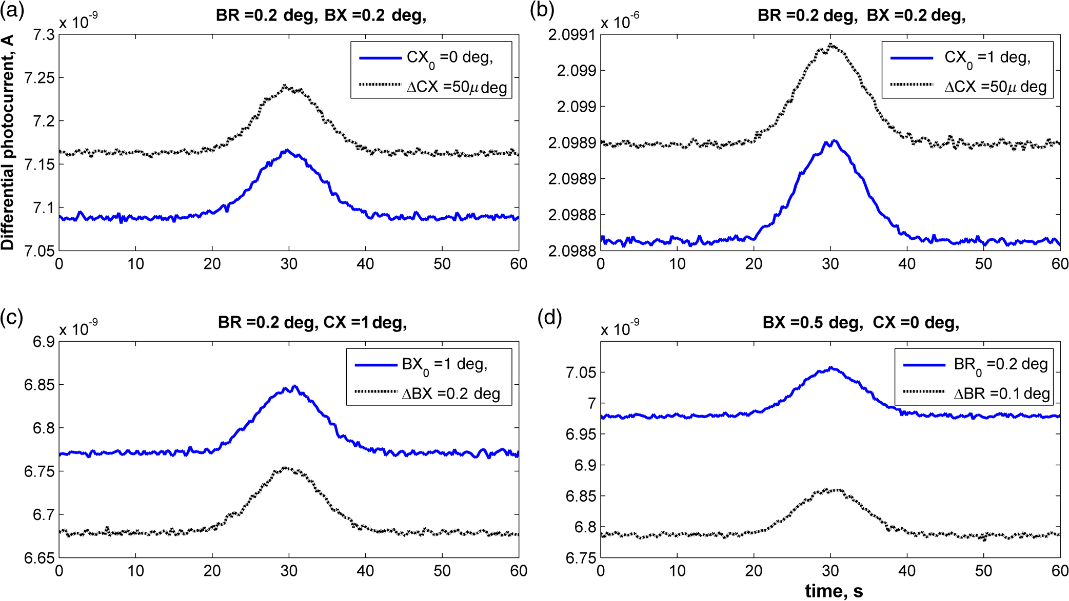

We can see by comparing (a) and (b) that misalignment of the EO crystal axial rotation by merely 1 deg causes a dramatic change in the signal level, increasing it by a factor of $2.1 \times 10^{- 6} / 7.1 \times 10^{- 9} \sim 295$ . Seemingly, this is a major problem. Normally, however, the polarimeter’s signal processing can be calibrated postproduction to account for this initial deviation—assuming it is fixed in time. However, we need to take into account an incremental misalignment that might be added during normal operation due to temperature changes. This incremental contribution is typically much smaller, yet it is unpredictable, and thus causes a measurement error. The effect of such incremental misalignment is described by the difference between the two lines in each subfigure.

To estimate the error, observe the plateau level on both sides of the pulse. We can see in (a) and (b) that when the EO crystal is misaligned with respect to the analyzer by an additive amount $Δ CX$ , the size of the resulting angular measurement error (the difference between the red and blue lines) is about the same as the size of this added misalignment. On the other hand, we can see in (c) and (d) that the polarimeter can tolerate considerably larger changes in BX and BR values than it can for the case of the EO crystal misalignment CX (recall the definition of these parameters in Fig. 2).

4. Analysis—Thermal Susceptibility

4.1.

Wavelength Sensitivity

There are three dominant effects that make the polarimeter wavelength sensitive. The first effect is the dispersion of the dynamic retardance of the EO retarder. The half-wavelength voltage of the retarder is given by

Eq. (9)

V_{π} = (\frac{λ}{2 r_{c 1} n_{z}^{3}}) (\frac{d_{EO}}{l_{EO}}),

where

λ

is the wavelength,

r_{c 1}

is the respective EO coefficient,

n_{z}

is the RI for

\hat{z}

-polarized wave, and

d_{EO}

and

l_{EO}

are the EO retarder thickness and length, respectively. As shown in Eq. (9), this voltage is proportional to the wavelength. When the wavelength drifts, and in the absence of accurate knowledge of the current wavelength, the reading of the actual

V_{0}

,

V_{π / 2}

becomes inaccurate and adds an error to the differential photocurrent. Furthermore, the presence of birefringence along the optical path accentuates this problem.

The second effect is the dispersion of the static retardance of the EO retarder. The refractive indices seen by the two linearly polarized waves propagating in the retarder, $n_{x, z}$ , are wavelength-dependent [i.e., $n_{x, z} (λ)$ ], as described by the respective Sellmeier equation (see Appendix B). If not corrected properly, this results in a substantial distortion of the differential photocurrent signal.

The third effect that results in wavelength sensitivity is Fabry–Perot interference that occurs between the input and output facets of the EO retarder. This effect modulates the transmissions of the two polarized wave components $\hat{x}, \hat{z}$ (in accordance with the directions in an $x$ -cut, $y$ -propagating EO retarder) independently as a function of wavelength, according to the well-known relation:

Eq. (10)

T_{x, z} = \frac{{(1 - R_{x, z})}^{2}}{1 + R_{x, z}^{2} - 2 R_{x, z} \cdot \cos (δ_{x, z})},

where

Eq. (11)

δ_{x, z} = \frac{4 π \cdot n_{x, z}}{λ} \cdot l_{EO} .

$R_{x, z}$ are the facet reflectivities for the two linear polarizations, and $T_{x, z}$ are introduced into the respective Jones matrices of the EO crystal (see Appendix A).

Direct monitoring of the wavelength, independently (of the photocurrent signal) and accurately (to the scale of 1 Å or less), can, in principle, help in compensating for these effects. But in reality, this poses a difficult technical task, particularly in the context of a miniaturized device. Thus, wavelength drift would result in a distortive effect on the photocurrent signal. In this subsection, this effect is estimated numerically.

For that purpose, a slight drift is added to the center wavelength at a constant rate $Δ λ / Δ t = 0.1 nm / \min$ . Thus, over the entire signal frame duration (i.e., 60 s in our example), the wavelength drifts by $Δ λ = 0.1 nm$ . The effect on the output signal (the differential photocurrent) is calculated for various birefringence scenarios and for various facet reflectivities at the EO retarder.

To distinguish between the contributions of these three effects, we recalculate the differential photocurrent for each case separately (i.e., with the other effects muted). The results are given in Figs. 12 Fig. 13–14.

Fig. 12

The effect of wavelength drift due to the dispersion of the dynamic retardance of the EO retarder. The calculated differential photocurrent versus time with the center wavelength drifting at a constant rate of $0.1 nm / \min$ . The facet reflectivities of the EO crystal are zero (so there is no Fabry–Perot effect), and the static retardance is nulled by imposing $n_{x} = n_{z}$ . To simplify, all birefringent components (optical windows, beam splitter) were assumed to have a similar axis, and BR and BX represent the total amount of birefringence (excluding the EO retarder) and the direction of this birefringence axis, respectively. The baseline and OA rotations were $α_{0} = 0.0048 \deg$ and $α_{pulse} = 50 μ \deg$ , respectively.

Fig. 13

The effect of wavelength drift due to the dispersion of the static retardance of the EO retarder. The calculated differential photocurrent versus time with the center wavelength drifting at a constant rate of $0.1 nm / \min$ . The facet reflectivities of the EO crystal are zero (so there is no Fabry–Perot effect) and the dynamic retardance is nulled by imposing $BX = BR = CX = 0$ . In these examples, the baseline and OA rotations were $α_{0} = 0.0048 \deg$ and $α_{pulse} = 20 m \deg$ , respectively.

Fig. 14

The effect of wavelength drift due to the Fabry–Perot interference between the EO retarder facets. The calculated differential photocurrent versus time with the center wavelength drifting at a constant rate of 0.33 nm/min. The dynamic and static retardances are nulled by imposing $BX = BR = CX = 0$ and $n_{x} = n_{z}$ , respectively. In these examples, the baseline and OA rotations were $α_{0} = 0.0048 \deg$ and $α_{pulse} = 240 μ \deg$ , respectively.

Figure 12 illustrates the effect of a wavelength drift, a change in $V_{π}$ with the wavelength, for two birefringence conditions: an ideal condition ( $BX = BR = CX = 0$ ) and an example of a medium-size misalignment condition ( $BX = BR = CX = 1 \deg$ ). The Fabry–Perot effect and the dispersion of the static retardance were muted by assigning zero-facet reflectivities ( $R_{x, z} = 0$ ) and imposing $n_{x} = n_{z}$ , respectively. The left graph shows that the signal is insensitive to wavelength drifts as long as no birefringence is present and the components are perfectly aligned. The right graph implies that for misalignment on the order of 1 deg, the signal is mildly sensitive to wavelength drifts on the order of a fraction of 1 nm.

Normally, for a well-designed polarimeter, 1 deg alignment accuracy is attainable in fabrication, and so the dynamic dispersion is not of major concern here.

The second effect, due to the wavelength dispersion of the static EO crystal retardance, is considerably larger. The conditions in this simulation were basically similar to the case above except for a much larger rotation pulse ( $a_{pulse} = 20 m \deg$ ), which was used to match the magnitude of the static effect. As in the previous case, the dynamic dispersion and the Fabry–Perot effect were muted by holding $V_{π}$ constant and assigning zero-facet reflectivities. An example is given in Fig. 13. The upper part shows the signal for the case where a single RTP crystal is used as an EO retarder. Clearly, the distortion effect is on the order of the OA rotation pulse, i.e., a few millidegrees.

This effect can be reduced by replacing the single crystal with a matched, orthogonal pair of RTP half-length crystals (lower part). Clearly, one cannot achieve a microdegree resolution by using a single crystal EO retarder.

The third effect, due to the Fabry–Perot interference that takes place within the crystal boundaries, has a different shape, which is periodical with the wavelength. It is also substantial in magnitude. Thus, note that in order to demonstrate it properly, a larger rotation pulse is used to simulate this case ( $α_{pulse} = 240 μ \deg$ ) than in the case of Fig. 12. The results are given in Fig. 14.

This interference effect superimposes an amplitude-modulated artifact on the signal. This artifact is periodical with the wavelength and has two periodicities: the faster (“carrier wave”) is due to Fabry–Perot interference. This periodicity represents a free spectral range (FSR) of $\sim 0.01 nm$ at the EO retarder. The slower (“envelope”) periodicity is due to the accumulating phase difference between $δ_{x}$ and $δ_{z}$ [see Eq. (11)] as a function of wavelength. As a result of this pattern, the magnitude of the error caused by the Fabry–Perot effect, which is mainly reflectivity dependent, is also wavelength dependent. For the purpose of assessment, one should normally refer to the worst-case scenario. As an example, for a facet reflectivity of 0.5%, it is apparent that the size of this noise effect is equivalent to $\sim 100 μ \deg$ or less (depending on the operating wavelength). This effect can be reduced in a number of ways. For example: (1) using a suitable antireflective coating; (2) polishing the crystal facets at a slight angle; (3) using a source that has a spectrum substantially wider than the EO retarder FSR, such as a visible vertical cavity surface emitting laser (VCSEL), or even a light-emitting diode (LED); and (4) removing the periodical artifact by a suitable signal processing.

We note that Fabry–Perot interference can also be caused by reflections from the two windows of the flow-cell, and can be taken into account and dealt with in a similar manner. It is, however, a weaker effect (mainly due to the lower RI difference), and it is thus not included in the current analysis.

4.2.

Thermal Susceptibility

A temperature drift typically leads to respective source wavelength changes (e.g., drift, mode hopping). These affect the output signal of the polarimeter (i.e., the differential photocurrent) via the mechanisms discussed in the previous subsection. In addition, the physical expansion of some of the optical components can similarly generate noise. For example, the expansion of the EO retarder can result in modulated transmission due to the Fabry–Perot effect. The expansion of the passive optical elements (optical windows and beam splitter) can change the contribution of these elements to the total birefringence.

Underlying the following calculation is an assumption that the temperature is uniform throughout the polarimeter, i.e., no thermal gradients are present. More specifically, regarding the various contributions mentioned above, we observe and assume the following:

• The thermal effect on the EO retardance can be minimized by using a matched, temperature-compensated, half-length retarder pair. In fact, we have implemented this solution in our experimental model and, therefore, its contribution to the total noise can be neglected.
• The thermally induced drift of the source wavelength is assumed to have a coefficient of $d λ / d T = 0.045 nm / ° C$ , which is typical of a visible VCSEL.
• With respect to the passive optical elements, we assume the following: (1) all elements are made of fused silica; (2) their birefringence is the maximal value given by the “Permissible optical path difference per cm glass path” in ISO 10110 part 2 for polarization optics,²⁴ which is $< 2 nm / cm$ between the two polarizations. For the working wavelength assumed here, this value gives a birefringence of $BR = 2 \times 2 π / 650 radians / cm$ glass. (3) The thermal expansion coefficient of fused silica (FS) is $6 \times 10^{- 7} / ° C$ ; (4) the total thickness of the passive optical elements (at $T_{0} = 20 ° C$ ) is $l_{FS} = 0.3 cm$ , i.e., $BR = 2 \times 2 π 0.3 / 650 radians$ ; and (5) there is an effective birefringence axis for the combination of these optical elements and it is aligned with the analyzer axis to within a range of BX deg.

To calculate the effect of these thermal contributions, we introduce the following temperature relations into the model:

Eq. (12)

BR (T) = \frac{2 \times 2 π}{λ (T)} \cdot l_{FS} \cdot [1 + α_{FS} (T - T_{0})],

Eq. (13)

λ (T) = λ_{0} + \frac{d λ}{d T} (T - T_{0}),

Eq. (14)

l_{EO} (T) = l_{EO} (T_{0}) \cdot [1 + α_{EO} (T - T_{0})],

where

T

is the temperature,

λ_{0} = 650 nm

, and

T_{0} = 20 ° C

. The temperature-dependent retarder transmissions

T_{x, z}

are calculated by using Eqs. (10) and (11) with the underlying notations

l_{EO} (T)

,

n_{x, z} (T)

, and

λ (T)

, where

n_{x, z} (T)

is calculated as detailed in Appendix B.

For the purpose of the following calculation, the temperature is linearly drifted over a time interval of 60 s. Some respective results, which demonstrate the thermally induced effect of the above described EO retarder mechanisms, are given in Fig. 15.

Fig. 15

The calculated differential photocurrent versus time with the ambient temperature center wavelength drifting at four constant $dT / dt$ rates. Various condition sets that relate to thermal effects taking place within the EO retarder are described. In all cases, $α_{0} = 0.0048 \deg$ , $α_{pulse} = 240 μ \deg$ , $CX = 0 \deg$ , and the EO retarder is made of a pair of matched orthogonal half-length retarders.

The results are given for four thermal drift rates ( $d T / d t = 0, 0.2, 0.5, 1 ° C / \min$ ). They represent, respectively, four temperature ranges: $Δ T = 0 ° C$ , $\pm 0.1 ° C$ , $\pm 0.25 ° C$ , and $\pm 0.5 ° C$ . For each rate, two facet reflectivities ( $R_{x} = 0.0005$ and 0.0025) are used.

It is evident that the larger the temperature drift is and the higher the facet reflectivities are, the more distorted the signal becomes. The temperature range of $\pm 0.25 ° C$ may be considered a typical condition within the human body, where the temperature is normally stable around 36.5 °C. In these cases, the periodical artifacts can easily be of the order of tens of microdegrees. Yet, if we recall that the OA-induced pulse height of $240 μ \deg$ is equivalent (for an optical path length of 10 mm) to a glucose pulse of $5 mg / dL$ , these thermally induced artifacts shall not preclude a reasonably accurate measurement of the glucose level.

5. Discussion: the Path to Better Polarimeter Performance and Miniaturization

There are several issues relevant to this task. Most important are aspects of sensitivity and stability, including (though not limited to) the LOD, physical dimensions and optomechanical tolerances, various thermal coefficients and the specifications of the light source, EO retarder, and electrical components.

The analysis given in the previous sections sheds light on some of these issues. Some implications of the above results are discussed briefly in this section, without getting into a detailed numerical analysis.

5.1.

Limit of Detection

For a polarimeter serving as a chiral detector in an HPLC system in the pharmaceutical industry, there is no lower bound for the LOD. The lower the LOD, the better, because it immediately means better and purer drugs. For a glucose sensor for diabetics, the minimal requirement to make it suitable to control an AP, with respect to the acceptable error, is $\pm 15 mg / dL$ .²¹ This puts a stringent requirement on the LOD, $\pm 15 mg / dL$ . For an optical path length of 10 mm, this translates into an optical rotation of $\pm 720 μ \deg$ . As was demonstrated above (see Fig. 8), the shot noise LOD for a 1-mW laser source is $\sim 10 μ \deg$ , i.e., 72 times smaller. This large difference leaves substantial room for those mechanisms that degrade the shot noise LOD, such as thermal drifts and optomechanical deviations.

5.2.

Physical Dimensions

The optical configuration is essentially flat and partially folded. The largest physical dimension is the length. The total length may be approximated by (see Fig. 1), assuming a 25% margin

Eq. (15)

l_{Pol} \approx (l_{light - source} + l_{polarizer} + l_{beam - splitter} + l_{flow - cell} + l_{EO}) \times 1.25 \approx (10 + 5 + 5 + 10 + 10) \times 1.25 \approx 50 mm .

This figure shows that our polarimeter can easily fit into almost any existing HPLC system, and an implantable polarimetric sensor would be viable in that respect.

5.3.

Light Source Considerations

In the above analysis, a monochromatic light source was assumed. In reality, a slight wavelength drift of such a source would induce a change of the output signal (see Figs. 12 Fig. 13–14). The dominant effect is the Fabry–Perot interference effect at the EO retarder, which would result in a respective noise (see Fig. 14). To reduce or even eliminate this noise effect, a low-coherence light source is preferred. The spectral width of this source should be much wider than the FSR of the EO retarder, which is (for a 10-mm long RTP crystal; see Fig. 14) $\sim 0.01 nm$ . In fact, we believe that this conclusion is more general and applicable to any polarimeter employing a laser light source and optical elements (such as a flow-cell and Faraday rotator) that allow for Fabry–Perot interference.

The light source (which operates CW) also needs to have an output power in the range of 1 mW and high power efficiency—to minimize heat dissipation and thermal effects. In this regard, a visible VCSEL or superluminescent LED would satisfy the above requirements.

5.4.

Thermal Considerations

A major issue is the effect of temperature instability. An internal stabilization mechanism would not be a problem for an HPLC chiral detector, but would be impractical in an implanted device in light of its small size, available temperature gradient, and very limited electrical power. On the other hand, the human body temperature is stabilized, normally to a range of few tenths of a degree Celsius. Thus, the question is: What magnitude of thermal uncertainty can the polarimeter tolerate? The analysis above shows (Fig. 15) that within a range of $\pm 0.25 ° C$ , and for a light source with a thermal coefficient of $d λ / d T = 0.045 nm / ° C$ (typical for a visible VCSEL), the differential photocurrent changes by an amount equivalent to only a few tens of microdegrees. Within a wider range of $\pm 0.5 \deg$ , the differential photocurrent may amount to an order of $100 μ \deg$ (still lower than the required LOD target of $\sim 720 μ \deg$ ). In either case, the magnitude of this effect can be reduced substantially by lowering the facet reflectivity of the EO and flow-cell windows to a fraction of a percent.

5.5.

Signal Detector Considerations

Two of the issues relevant to the polarimeter’s signal detector are the detectivity parameters (that determine the angular LOD) and the required dynamic range (because the small signal superposes a substantial background level). We assume a noncooled detector, particularly in the context of an implanted device, where the physical space and electrical current are very limited. In the case of an HPLC system, cooling might be an option.

The sensor assumed for the analysis above (S 1226-18BQ, Hamamatsu), is a commercially available small, light detector that is not the state-of-the-art in this field. Nonetheless, the calculated shot-noise limit of the angular LOD is $\sim 10 μ \deg$ (see Fig. 8), which is almost two orders of magnitude better than the clinically induced requirement.

With respect to the required dynamic range, it was calculated above (see Fig. 9) to be lower than 10⁶. This requirement is within the capability of several Si photodiodes.

5.6.

Some EO Retarder Considerations

One conclusion from the above analysis is that the EO retarder must be temperature-compensated in order to achieve accuracy of few tens of microdegrees. This somewhat complicates the application of the retarder, but can certainly be done.

Two other issues relevant to the EO retarder are the amplitude of the modulating voltage waveform and the physical dimensions of the retarder. These two are linked [see Eq. (9)]. The half-wavelength voltage can be reduced by using a shorter wavelength and/or by using a lower thickness-to-length ratio. In fact, a shorter wavelength is doubly beneficial in that respect, as it results in lower diffraction and thus facilitates a lower thickness-to-length ratio, roughly in proportion. By this argument, it is possible, in principle, to reduce the modulation peak voltage, which is currently $V_{π / 2} \sim 240 V$ , roughly in proportion to the operating wavelength squared.

5.7.

Optomechanical Tolerances

The effects of three types of optomechanical misalignments were considered in detail in this article: CX—the angular misalignment of the EO retarder, BX—the effective misalignment of the passive optical elements along the optical path (which were assumed to have an effective birefringence phase BR), and PX—the deviation of the polarizer axis from its ideal position. Of these, CX is the most critical parameter, and, roughly speaking, adds angular error of similar magnitude (as the OA-induced rotation). The tolerance on BX is more relaxed, on the order of few tens of a degree. PX is also a noncritical parameter, and can be controlled to within an angular deviation of one degree. In any case, a slight error in setting PX would mainly affect the magnitude of the signal, and much less the accuracy of the polarimeter.

6. Conclusion

The detailed analysis in this article demonstrates the advantages inherent to the design of our OR polarimeter—namely its small size and noise rejection capability. The current resolution and accuracy of this polarimeter equal, and sometimes even surpass, that of the best available commercial OR polarimeters. Its unique ability to efficiently reject PR artifacts, which is not shared by any other OR polarimeter, makes it especially attractive for HPLC analyses in the pharmaceutical industry. The ability to miniaturize it to the size of a pacemaker opens the door for its future use as a chronically implanted CGM for diabetics and a viable alternative to current enzyme-based CGMs.

This article also lays out the path to further improvements to the polarimeter’s performance. Some of these improvements, mainly in the control of wavelength drift, are currently underway and show promise to enable substantial increase in the polarimeter’s resolution and accuracy.

Appendices

Appendix A:

Component Jones Matrices

The Jones matrices that apply to the various components along the optical path are as follows.

The analyzer matrix is

[A n] = (\begin{matrix} \cos θ_{A n} & \sin θ_{A n} \\ - \sin θ_{A n} & \cos θ_{A n} \end{matrix}) \cdot (\begin{matrix} t_{x} & 0 \\ 0 & t_{z} \end{matrix}) \cdot {(\begin{matrix} \cos θ_{A n} & \sin θ_{A n} \\ - \sin θ_{A n} & \cos θ_{A n} \end{matrix})}^{- 1},

where

θ_{A n}

is the angle of the analyzer transmission axis with respect to the

x

-axis. It is assumed that the analyzer passes the vertical polarization (i.e., directed at the

z

-axis),

t_{x, z}

refers to the

E

-field transmission, and

20 \log_{10} (t_{x} / t_{z}) = ER

is the ER of the analyzer (and the polarizer).

Similarly, for the other optical components

[{BS}_{ref}] = (\begin{matrix} \cos θ_{BS ref} & \sin θ_{BSref} \\ - \sin θ_{BS ref} & \cos θ BSref \end{matrix}) \cdot (\begin{matrix} e^{i ϕ_{BS ref} / 2} & 0 \\ 0 & e^{- i ϕ_{BS ref} / 2} \end{matrix}) \cdot {(\begin{matrix} \cos θ_{BS ref} & \sin θ_{BS ref} \\ - \sin θ_{BS ref} & \cos θ_{BS ref} \end{matrix})}^{- 1}, [{FC}_{in}] = (\begin{matrix} \cos θ_{FC in} & \sin θ_{FC in} \\ - \sin θ_{FC in} & {\cos θ}_{FC in} \end{matrix}) \cdot (\begin{matrix} e^{i ϕ_{FC in} / 2} & 0 \\ 0 & e^{- i ϕ_{FC in} / 2} \end{matrix}) \cdot {(\begin{matrix} \cos θ_{FC in} & \sin θ_{FC in} \\ - \sin θ_{FC in} & \cos θ_{FC in} \end{matrix})}^{- 1}, [{OA}_{left}] = (\begin{matrix} \cos α & \sin α \\ - \sin α & \cos α \end{matrix}), [{FC}_{out}] = (\begin{matrix} \cos θ_{FC out} & \sin θ_{FC out} \\ - \sin θ_{FC out} & \cos θ_{FC out} \end{matrix}) \cdot (\begin{matrix} e^{i ϕ_{FC out} / 2} & 0 \\ 0 & e^{- i ϕ_{FC out} / 2} \end{matrix}) \cdot {(\begin{matrix} \cos θ_{FC out} & \sin θ_{FC out} \\ - \sin θ_{FC out} & \cos θ_{FC out} \end{matrix})}^{- 1}, [{EO}_{1}] = (\begin{matrix} \cos θ_{EO} & \sin θ_{EO} \\ - \sin θ_{EO} & \cos θ_{EO} \end{matrix}) \cdot (\begin{matrix} \sqrt{T_{x}} \cdot e^{i (ϕ_{EO} / 2 + π (n_{x} - n_{z}) l_{EO} / λ)} & 0 \\ 0 & \sqrt{T_{z}} \cdot e^{- i (ϕ_{EO} / 2 + π (n_{x} - n_{z}) l_{EO} / λ)} \end{matrix}) \cdot {(\begin{matrix} \cos θ_{EO} & \sin θ_{EO} \\ - \sin θ_{EO} & \cos θ_{EO} \end{matrix})}^{- 1},

[Mirror] = (\begin{matrix} 1 & 0 \\ 0 & - 1 \end{matrix}), [{EO}_{2}] = [{EO}_{1}], [{OA}_{right}] = {[{OA}_{left}]}^{- 1} = (\begin{matrix} \cos α & - \sin α \\ \sin α & \cos α \end{matrix}), [{BS}_{pass}] = (\begin{matrix} \cos θ_{BS pass} & \sin θ_{BS pass} \\ - \sin θ_{BS pass} & \cos θ_{BS pass} \end{matrix}) \cdot (\begin{matrix} e^{i ϕ_{BS ref} / 2} & 0 \\ 0 & e^{- i ϕ_{BS ref} / 2} \end{matrix}) \cdot {(\begin{matrix} \cos θ_{BS pass} & \sin θ_{BS pass} \\ - \sin θ_{BS pass} & \cos θ_{BS pass} \end{matrix})}^{- 1}, [Pol] = (\begin{matrix} \cos θ_{Pol} & \sin θ_{Pol} \\ - \sin θ_{Pol} & \cos θ_{Pol} \end{matrix}) \cdot (\begin{matrix} t_{x} & 0 \\ 0 & t_{z} \end{matrix}) \cdot {(\begin{matrix} \cos θ_{Pol} & \sin θ_{Pol} \\ - \sin θ_{Pol} & \cos θ_{Pol} \end{matrix})}^{- 1}, (\begin{matrix} E_{x}^{source} \\ E_{y}^{source} \end{matrix}) = (\begin{matrix} 0 \\ 1 \end{matrix}),

where BS, FC, OA, EO, and Pol stand for the beam splitter, flow-cell, optical activity, EO retarder, and polarizer, respectively.

θ

and

ϕ

stand for the rotation angle of the component axis with respect to the

x

-axis and the birefringence-induced phase shift between the two orthogonal polarization components, respectively.

Appendix B: Relevant Numerical/Physical Data

B1.

Photodiode Parameters

In the calculation above, we used the parameters of a specific Si photo diode (S 1226-18BQ, Hamamatsu). The values and universal constants are as follows:²³

I_{dark} = 2 \cdot 10^{- 12} A, R_{sh} = 20 G Ω, B W_{n} = 10 Hz, R_{λ = 650 nm} = 0.33 A / W, k_{B} = 1.38 \times 10^{- 23} m^{2} {kgs}^{- 2} K^{- 1}, q_{e} = 1.60217657 \times 10^{- 19} coulombs .

B2.

Dispersion Relations

The EO retarder in our polarimeter²² was made of an $x$ -cut, $y$ -propagating, RTP ( ${RbTiOPO}_{4}$ ) crystal (Raicol Crystals Ltd.). The electrodes were placed perpendicular to the $z$ -axis (with spacing $d_{EO} = 2 mm$ ), to facilitate using the $r_{33}$ EO tensor component. Sellmeier relations for RTP crystals, as well as their temperature dependence, are documented in the literature.²⁵^,²⁶ In particular, the temperature-dependent dispersion relations of RTP as reported recently are as follows:²⁵

n_{x}^{2} = 4.65575 + \frac{0.04068}{λ^{2} - 0.04750} + \frac{204.2586}{λ^{2} - 130.7684}, n_{z}^{2} = 7.97109 + \frac{0.06079}{λ^{2} - 0.05968} + \frac{1234.6913}{λ^{2} - 269.8094},

where

λ

is in microns. The temperature dependence was given by

\frac{d n_{x}}{d T} = (\frac{0.1227}{λ^{3}} - \frac{0.3064}{λ^{2}} + \frac{0.4469}{λ} + 0.0941) \times 10^{- 5} ({\deg C}^{- 1}), \frac{d n_{z}}{d T} = (\frac{1.1823}{λ^{3}} - \frac{2.8099}{λ^{2}} + \frac{2.6613}{λ} + 0.1415) \times 10^{- 5} .

B3.

Optical Component Parameters

Throughout the article, the basic set of parameter values used in the calculations is as follows:

λ = 650 nm, {ER}_{polarizer} = {ER}_{analyzer} = 40 dB, l_{EO} = 10 mm, d_{EO} = 2 mm, α_{EO} = 1.1 \times 10^{- 5} 1 / \deg C (RTP), α_{FS} = 0.4 \times 10^{- 5} 1 / \deg C .

References

1.

Rudolph Research Analytical—products website, “Polarimetry–industry applications,” (2015) http://rudolphresearch.com/products/polarimeters/polarimetry-definitions/ ( January ). 2015). Google Scholar

2.

“FDA’s policy statement for the development of new stereoisomeric drugs,” Chirality, 4 338 –340 (1992). http://dx.doi.org/10.1002/chir.530040513 CHRLEP 1520-636X Google Scholar

3.

Y. Zhang et al., “Enantioselective chromatography in drug discovery,” Drug Discov. Today, 10 (8), 571 –577 (2005). http://dx.doi.org/10.1016/S1359-6446(05)03407-0 DDTOFS 1359-6446 Google Scholar

4.

C. F. So et al., “Recent advances in noninvasive glucose monitoring,” Med. Devices (Auckl), 5 45 –52 (2012). http://dx.doi.org/10.2147/MDER.S28134 Google Scholar

5.

O. S. Khalil, “Non-invasive glucose measurement technologies: an update from 1999 to the dawn of the new millennium,” Diabetes Technol. Ther., 6 660 –697 (2004). http://dx.doi.org/10.1089/dia.2004.6.660 Google Scholar

6.

J. W. Gilbert, H. C. Weiser and F. P. Holladay, “A cerebrospinal fluid glucose biosensor for diabetes mellitus,” ASAIO J., 38 82 –87 (1992). http://dx.doi.org/10.1097/00002480-199204000-00003 Google Scholar

7.

E. J. Gillham, “A high-precision photoelectric polarimeter,” J. Sci. Instrum., 34 435 –439 (1957). http://dx.doi.org/10.1088/0950-7671/34/11/302 JSINAY 0368-4253 Google Scholar

8.

E. S. Yeung et al., “Detector based on optical activity for high performance liquid chromatographic detection of trace organics,” Anal. Chem., 52 1399 –1402 (1980). http://dx.doi.org/10.1021/ac50059a006 ANCHAM 0003-2700 Google Scholar

9.

R. Däppen et al., “Aspects of quantitative determinations with polarimetric detectors in liquid chromatography,” Anal. Chim. Acta, 282 47 –54 (1993). http://dx.doi.org/10.1016/0003-2670(93)80350-T ACACAM 0003-2670 Google Scholar

10.

F. G. Sanchez, A. N. Diaz and I. M. Lama, “Polarimetric detection in liquid chromatography: an approach to correct refractive index artefacts,” J. Liq. Chromatogr. Relat. Technol., 31 3115 –3131 (2008). http://dx.doi.org/10.1080/10826070802480057 Google Scholar

11.

Rudolph Research Analytical—polarimeters website, “Autopol polarimeter footprint chart,” (2015) http://rudolphresearch.com/autopol-polarimeter-sizing-chart-1/ ( January ). 2015). Google Scholar

12.

H.-J. King et al., “Concentration measurements in chiral media using optical heterodyne polarimeter,” Opt. Commun., 110 259 –262 (1994). http://dx.doi.org/10.1016/0030-4018(94)90422-7 OPCOB8 0030-4018 Google Scholar

13.

T. Mitsui and K. Sakurai, “Microdegree azimuth polarimeter using optical heterodyne detection,” Jpn. J. Appl. Phys., 35 4844 –4847 (1996). http://dx.doi.org/10.1143/JJAP.35.4844 Google Scholar

14.

C. Chou, “A phase sensitive optical rotation measurement in a scattered chiral medium using a Zeeman laser,” Opt. Commun., 230 259 (2004). http://dx.doi.org/10.1016/j.optcom.2003.11.055 OPCOB8 0030-4018 Google Scholar

15.

C. Chou et al., “Polarized photon-pairs heterodyne polarimetry for ultrasensitive optical activity detection of a chiral medium,” J. Phys. Chem. B, 111 9919 –9922 (2007). http://dx.doi.org/10.1021/jp0689058 JPCBFK 1520-6106 Google Scholar

16.

J.-F. Lin et al., “A new electro-optic modulated circular heterodyne interferometer for measuring the rotation angle in a chiral medium,” Opt. Lasers Eng., 47 39 –44 (2009). http://dx.doi.org/10.1016/j.optlaseng.2008.08.004 OLENDN 0143-8166 Google Scholar

17.

J.-Y. Lee and D.-C. Su, “Improved common-path optical heterodyne interferometer for measuring small optical rotation angle of chiral medium,” Opt. Commun., 256 337 –341 (2005). http://dx.doi.org/10.1016/j.optcom.2005.06.056 OPCOB8 0030-4018 Google Scholar

18.

L. Bougas et al., “Chiral cavity ring down polarimetry: chirality and magnetometry measurements using signal reversals,” J. Chem. Phys., 143 104202 (2015). http://dx.doi.org/10.1063/1.4930109 JCPSA6 0021-9606 Google Scholar

19.

V. Evtuhov and A. E. Siegman, “A “twisted-mode” technique for obtaining axially uniform energy density in a laser cavity,” Appl. Opt., 4 142 –143 (1965). http://dx.doi.org/10.1364/AO.4.000142 APOPAI 0003-6935 Google Scholar

20.

J. Poirson et al., “Resonant cavity gas-phase polarimeter,” Anal. Chem., 70 4636 –4639 (1998). http://dx.doi.org/10.1021/ac980286e ANCHAM 0003-2700 Google Scholar

21.

ISO 15197:2013, “In vitro diagnostic test systems—requirements for blood-glucose monitoring systems for self-testing in managing diabetes mellitus,” (2013) http://www.iso.org/iso/catalogue_detail?csnumber=54976 Google Scholar

22.

D. Goldberg and Z. Weissman, “Compact, high-resolution, self-referenced, optical activity polarimeter for high-pressure liquid chromatography systems,” Appl. Opt., 53 577 –587 (2014). http://dx.doi.org/10.1364/AO.53.000577 APOPAI 0003-6935 Google Scholar

23.

D. H. Goldstein, Polarized Light, CRC Press, Boca Raton (2003). Google Scholar

24.

ISO 10110-2:1996, “Optics and optical instruments—preparation of drawings for optical elements and systems—part 2: material imperfections—stress birefringence,” (1996) http://www.iso.org/iso/iso_catalogue/catalogue_tc/catalogue_detail.htm?csnumber=18089 Google Scholar

25.

T. Mikami, T. Okamoto and K. Kato, “Sellmeier and thermo-optic dispersion formulas for RbTiOPO4,” Opt. Mater., 31 1628 –1630 (2009). http://dx.doi.org/10.1016/j.optmat.2009.03.012 Google Scholar

26.

I. Yutsis, B. Kirshner and A. Arie, “Temperature-dependent dispersion relations for RbTiOPO₄ and

{RbTiOAsO}_{4}

,” Appl. Phys. B, 79 77 –81 (2004). http://dx.doi.org/10.1007/s00340-004-1498-2 Google Scholar

Biography

Zeev Weissman is currently a staff member at the Department of Electrical Engineering, Shenkar College of Engineering and Design. He holds a BSc degree in electrical engineering from the Technion in Haifa, Israel, and MSc and PhD degrees in engineering from Tel Aviv University. His research interests are in optical waveguide devices and optical polarimetry for biomedical applications.

Doron Goldberg is a researcher at the MIGAL Galilee Research Institute, where he develops optical sensors for analytical and biomedical applications. He is also a staff member and senior lecturer at the Tel-Hai Academic College. He holds a BSc degree from the Department of Biochemistry and Human Nourishment, the Faculty of Agriculture at the Hebrew University (Cum laude), MSc (summa cum laude), and PhD degrees from the Department of Biochemistry, Hebrew University, Jerusalem.

CC BY: © The Authors. Published by SPIE under a Creative Commons Attribution 4.0 Unported License. Distribution or reproduction of this work in whole or in part requires full attribution of the original publication, including its DOI.

Citation Download Citation

Zeev Weissman and Doron Goldberg "Self-referenced, microdegree, optical rotation polarimeter for biomedical applications: an analysis," Journal of Biomedical Optics 21(7), 071104 (22 December 2015). https://doi.org/10.1117/1.JBO.21.7.071104

Published: 22 December 2015

Access the abstract

JOURNAL ARTICLE
16 PAGES

DOWNLOAD PAPER SAVE TO MY LIBRARY