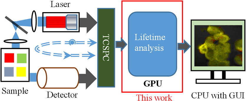
1.

Introduction

Fluorescence lifetime imaging microscopy (FLIM) is a powerful imaging technique that can not only locate fluorescent molecules (fluorophores) but also provide images based on the temporal decay rate of the fluorescence emitted from fluorophores. In contrast to traditional intensity imaging, FLIM is insensitive to the intensities of light sources and probe concentrations.¹ As lifetime characteristics of fluorophores are usually sensitive to their environment, FLIM can image physiological parameters such as pH, O₂, Ca²⁺, Cl⁻, or temperature linked to diseases or potential therapies. For example, FLIM has been combined with Förster resonance energy transfer (FRET) techniques (FLIM-FRET) for assessing drug efficacy and clearance in tumors,² cellular temperature in cancerous tissues under treatments,³ and cerebral energy metabolism for understanding brain functions.⁴

In order to monitor fast dynamic biological events, it is necessary to build a high-speed or even real-time FLIM system.^5–7 FLIM can operate in the time domain or frequency domain.^8,9 Wide-field frequency-domain FLIM instruments are capable of capturing phase images at a high frame rate, but the acquisition will decrease if more than 10 phase images are required (which usually happens in realistic laboratory scenarios), and accurate analysis heavily relies on appropriate software.¹⁰ Moreover, if there is more than one decay component in a fluorescence histogram, excitations at multiple frequencies¹¹ or at a single frequency with a sufficiently narrow pulse (using higher-order harmonic frequencies) are required,¹² greatly reducing the acquisition rate and increasing the system complexity. Time-domain techniques, on the other hand, include gated camera¹³ and time-correlated single-photon counting (TCSPC) methods. Due to superior temporal resolution and recent developments in advanced laser sources and cameras, TCSPC techniques have been the gold standard solutions for FLIM experiments.^14–16 Traditional photomultiplier tube (PMT) based TCSPC instruments are capable of single-photon detection, and they can have multiple channels to boost the acquisition. The latest multichannel TCSPC systems^16–19 can acquire image raw data in seconds, but the FLIM images are mainly processed by slow analysis software. Recent advances in semiconductor technologies have allowed single-photon detectors to be fabricated in two-dimensional (2-D) arrays in a low-cost silicon process with integrated on-chip TCSPC modules.^20–22 These highly parallel single-photon avalanche diode (SPAD) arrays can be configured for wide-field or multifocal multiphoton microscopy systems to enhance the acquisition rate.¹⁶ Faster acquisition means more image raw data are generated in a shorter period of time. Similar to the multi-PMT TCSPC system, 2-D SPAD+TCSPC arrays in a single chip significantly enhance the parallelism, enabling real-time acquisition.^21,23 And the data throughput of the latest 2-D SPAD arrays can easily exceed tens of gigabit/s, imposing significant challenges in data handling and image analysis.²¹ In such systems, lifetime analysis has become a bottleneck for real-time FLIM applications.

To address this problem, several noniterative fast FLIM algorithms have been developed, including rapid lifetime determination (RLD),^24,25 the integral equation method (IEM),²⁶ the center of mass method (CMM),^23,27 the phasor method (PM),^28,29 moment methods,³⁰ and fast bi-exponential solvers, including bi-exponential centre of mass method (BCMM)³¹ and the four-gate method.³² To boost image generation, high-performance hardware can be employed to process the imaging data. For example, Li et al. have previously implemented field programmable gate array (FPGA) embedded FLIM processors capable of offering video-rate FLIM imaging.²³ These hardware embedded FLIM processors, however, only generate single-exponential FLIM images and are less flexible than traditional iterative algorithms, such as maximum likelihood estimation (MLE),³³ the least square method (LSM),^33,34 and global analysis (GA).^35–37 Compared with noniterative methods, iterative algorithms have the following advantages: (1) they have a wider working range, so that they can be employed in most situations; (2) they can support bi- or multiexponential analysis; and (3) they have better precision and accuracy performances. But iterative algorithms are generally slow and cannot be sped-up easily, and are also difficult to realize in hardware.

In this paper, we will focus on how the latest graphics processing units (GPUs) can be used to increase the lifetime estimation speed for both noniterative and iterative algorithms. The work developed in this paper can be a fast FLIM processor between the SPAD-array or multi-PMT acquisition front-ends and the GPU shown in Fig. 1. The realization of parallel FLIM analysis and its optimization will be given in Sec. 2, including a brief introduction of the algorithms. In Sec. 3, we will compare the GPU analysis with CPU parallel analysis and verify the new GPU FLIM analysis methods on both synthesized data and experimental data.

Fig. 1

Focus of this paper in assumed FLIM system.

2.

Methodology

To generate a lifetime image requires a FLIM analysis algorithm to process a large number of pixels with each pixel containing a decay histogram. Instead of calculating lifetimes in a pixel-by-pixel manner, it is desirable to analyze all histograms in parallel for real-time applications. Although FPGA technologies have already been introduced in this emerging area,³⁸ their usage is still limited since only the hardware-friendly algorithms, such as RLD, IEM, and CMM,^23–27 can be implemented. GPUs, on the other hand, contain a massive number of cores, offering significant computing power, and allow more complex algorithms for data analysis. Therefore, GPUs show great potential in real-time FLIM applications.

2.3.

Graphic Processing Unit Implementation

All the algorithms introduced above can be translated into GPU programs using the CUDA application programming interfaces.^46–48 In this section, we describe how to implement noniterative and iterative algorithms on GPUs. From this section, one can also understand why a GPU works faster than a CPU.

We assume the FLIM image to be analyzed contains $512\times 512\text{pixels}$, and the histogram in each pixel has 256 time bins. In GPU programming, the program is launched as grids of blocks of threads (the left-hand charts of Figs. 2 and 3 show the relationships among thread, block, and grid).⁴⁷ And instead of being executed only once or a few times in a regular C program, it is executed $N$ times in parallel by $N$ different CUDA threads.⁴⁷

Fig. 2

Relationships among thread, block, and grid, and GPU implementation of noniterative algorithms for FLIM analysis.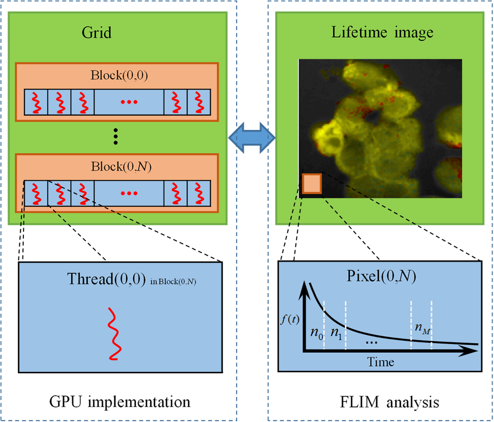

Fig. 3

Relationships among thread, block, and grid, and GPU implementation of iterative algorithms for FLIM analysis.

2.3.1.

Thread-based computing for noniterative algorithms

For noniterative algorithms, GPU and CPU programs share similar code, except for the specific configurations of hardware resources and memory accesses in GPU implementations. The histogram of each pixel is analyzed by an independent CUDA thread, as shown in Fig. 2, and each block contains 512 threads. This configuration allows analyzing a large number of pixels simultaneously, the exact number being determined by the number of streaming multiprocessors (SMPs). In this case, up to 30,720 pixels can be launched on the NVIDIA Tesla K40 GPU.⁴⁷ Then, following the single instruction multiple threads mechanics,⁴⁹ the lifetime estimations can be realized in parallel, instead of calculating lifetimes in a serial pixel-by-pixel manner as on a CPU.

2.3.2.

Block-based computing for iterative algorithms

For iterative algorithms, the histogram for each pixel is analyzed by a separate CUDA block, as shown in Fig. 3 (here, each thread processes a single time bin, instead of an entire pixel as in noniterative algorithms), and each such block contains 256 threads that correspond to the 256 time bins. This configuration still also allows a quite large number of pixels to be analyzed simultaneously, and 120 pixels are expected on the NVIDIA Tesla K40. Here, we take LSM as an example to demonstrate how to implement iterative algorithms on GPUs. The CUDA operations can be divided into the following two categories.

Thread-independent operation

For those operations that are independent in each time bin, the CUDA provides a basic instruction. For example, subtraction or division for each time bin $(N_j-Y_j)/{\sigma }_j$ can be finished in only one instruction cycle of one instruction as shown in Fig. 4(a) (here, we just take subtraction as an example, since division follows the same procedure), whereas there are 64 subtraction cycles in the CPU-OpenMP operation [Fig. 4(b)]. In Fig. 4(a), $N_j$ and $Y_j$ are stored in the variables SubA and SubB, respectively, and every thread has these two variables, whereas the CPU defines two arrays (SubA[256] and SubB[256]) for loop operations.

Fig. 4

Subtraction in GPU and CPU-OpenMP processing.

Thread-exchanged operation

Alternatively, the CUDA provides a special solution for some operations where communication or data sharing with other time bins (threads) is necessary. As shown in Fig. 5(a),^50,51 the data ${(N_j-Y_j)}^2/{\sigma }_j^2$ of each time bin is stored in the $j$th element of a shared memory array SumA (shared memory is on-chip high-speed memory, which enables the threads in the same block to access the same memory content; arrays are defined by: __shared__ SumA[256], in CUDA programming⁴⁷). In step 1, the first $256/2=128$ threads compress the array SumA into 128 elements by combining the $j$th and ($j+128$)th units ($j=1,\dots ,128$) simultaneously, followed by several similar steps. Finally, after only ${\log }_{2}256=8$ steps (it is not a requirement that the number of threads in a block has to be a power of 2, but it maximizes performance), the summation reduction result can be acquired, instead of after 65 steps in the CPU-OpenMP version as shown in Fig. 5(b).

Fig. 5

Summation reduction in GPU and CPU processing.

2.4.

Optimization of Graphic Processing Unit Programming

In order to maximize the ability of the GPU in FLIM analysis, it is necessary to consider the specifications of GPU hardware, manage the memory properly, and design a specific programming strategy for each individual algorithm. The following considerations are mainly for iterative algorithms, except the kernel configuration and overlap of data transfer, which are also applicable to noniterative algorithms.

2.4.1.

Kernel configuration

When we launch the kernel in a host (CPU), which is the entrance to GPU processing, similar to the main function in the C language, a proper size of block (determining how many threads in a block) and grid (determining the number of blocks) should be given in order to optimize the GPU performance. On CUDA GPUs, 32 threads are bound together into a so-called warp, which is executed in lockstep. Accordingly, it is suggested that the number of time bins should be a multiple of 32, for instance, 256. Furthermore, according to the GPU hardware specification, at most 2048 threads or 16 blocks can be launched in an SMP, which is the workhorse of the GPU⁴⁶ and puts a different constraint on the number of threads. Table 3 illustrates that for thread numbers that are not multiples of 32, although fewer threads are launched, the processing time can be longer. This is due to the so-called warp divergence, which occurs if threads in the same warp follow different conditional branches in the code. In CUDA, diverging threads in a warp are executed serially, and branch divergences therefore lead to considerably slower execution. Additionally, when the thread number is 224, although it is a multiple of 32, its operation time is longer than expected: $1662.5>(224/256)\times 1870.2=1636.4\mathrm{ms}$. This is because for each SM, only $2016(<2048)$ threads have been launched, so that not all the hardware resources are being used.

Table 3

Operation time under different block size of LSM graphic processing unit (GPU).

Threads per block	Warp divergence	Full launch	Time (ms)	Time/bin (ms)
256	No	Yes	1870.2	7.305
255	Yes	No	1898.9	7.447
253	Yes	No	1912.8	7.560
250	Yes	No	1914.2	7.657
225	Yes	No	1960.4	8.713
224	No	No	1662.5	7.422

In this case, considering a $512\times 512$ FLIM image to be generated, we examine the performance of GPU FLIM with a different grid size. As shown in Table 4, for FLIM analysis, the calculation times for different sizes are almost the same, so there is no need to configure the block dimension as long as it follows the limitation (maximum grid size of NVIDIA K40: $⟨2^{31}-1,65,535,65535⟩$⁴⁷).

Table 4

Operation time under different grid size of LSM-GPU.

First dimension	Second dimension	Time (ms)
$512\times 512$	1	1869.4
$512\times 16$	32	1867.2
$512\times 2$	256	1871.3
512	512	1870.2
32	$16\times 512$	1872.6
2	$256\times 512$	1870.7

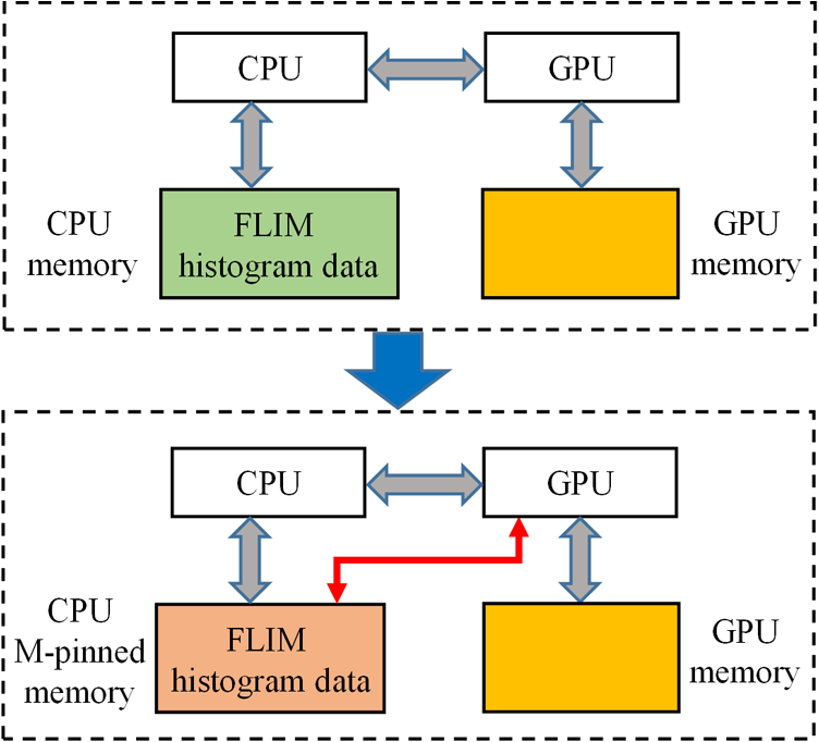
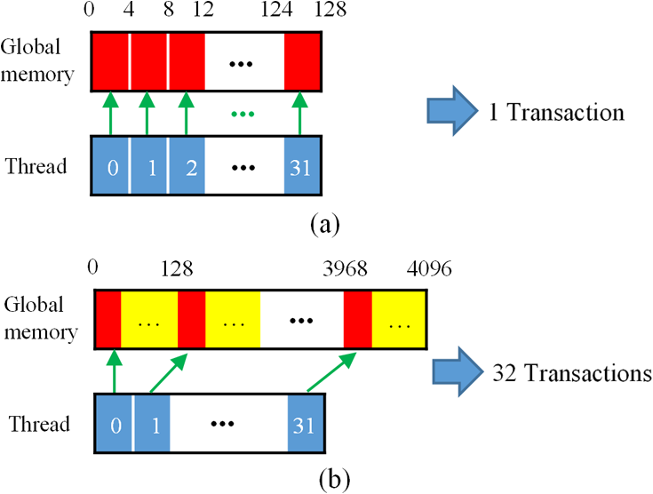
Although simple algorithms use different configurations (i.e., different size of grid or block), the same features can be found as illustrated above.

2.4.2.

Memory optimization

In order to achieve higher performance, it is necessary to optimize the memory usage and maximize the memory throughput. For FLIM analysis, three aspects should be considered as follows.

First, for a real-time FLIM process, the GPU has to access the histogram data from the CPU for every image frame, so mapped pinned (M-pinned) memory should be encouraged, which is the host memory and has been page-locked and mapped for direct access by the GPU, as shown in Fig. 6.⁴⁶ Also, to minimize data transfers between the host (CPU) and device (GPU), the GPU FLIM analysis only uses device memory once the histogram data have been transferred from the host.

Fig. 6

GPU-FLIM analysis with mapped pinned memory.

Moreover, when a large amount of data is used, it is important to consider asynchronous and overlapping transfers with computations.⁵² CUDA streams (which are sequences of operations that are performed in order on the device) can be used to fulfill this mission. As shown in Fig. 7(a), in sequential mode, the kernel can only be launched after all the data have been transferred to the GPU memory. In contrast, for the concurrent mode, the pixels of an FLIM image are divided into several groups, and each pixel within the same group will be launched in the same stream. As illustrated in Fig. 7(b), histogram or lifetime data transfer and calculation kernels are separated into different streams. This configuration allows data transfer and kernel execution to run simultaneously, and can reduce the whole processing time measurably.

Fig. 7

Timeline comparison of (a) sequential and (b) concurrent executions.

Last but not least, GPUs have several memory spaces including the shared, global, constant, texture, register, and local memory,^47,52 and for GPU performance, the most important area is memory management.⁵² Among these memories, the shared memory is on-chip memory, and it has much higher bandwidth and much lower latency than the local or global memory. It is highly recommended that the shared memory should be used as much as possible, especially when there is communication between threads in the same block (e.g., summation reduction operations). However, shared memory is very limited in size, and it is unavoidable to use the large global memory. Because this is by far the slowest memory accessible from the GPU, care should be taken to access it in the most efficient way. CUDA supports so-called coalesced memory access, where several threads of a warp access a congruent area of device memory in a single memory fetch. Using coalesced access as much as possible is very important to minimize the necessary bandwidth. Figure 8 illustrates the difference between the coalesced access and noncoalesced access, and the ensuing large speed difference.^47,53 To be specific, this implies, for example, that for noniterative algorithms, the histogram data need to be arranged such that the data of the same time bin but different pixels are directly adjacent, since each thread will access data of the same time bin of the corresponding pixel. For iterative algorithms, however, data of each time bin of a pixel have to be stored in continuous memory locations. Besides, the constant and texture (optimized for 2-D spatial locality) memory spaces, which are cached and read only, can be used to save constant arrays or matrices used in the algorithm and can also speed up the processing. For example, for IEM, every pixel uses the same coefficients $C_j$, and we can calculate the value before processing, so $C_j$ can be kept in the constant memory (declared by “__constant__ float CoIEM[]”).

Fig. 8

Global memory access: (a) coalesced access and (b) noncoalesced access.

2.4.3.

Programming strategies

The first consideration is to trade the precision for the speed when it does not affect the result, such as using single-precision operations instead of double-precision ones. Then the number of divergent warps (threads in the same warp have different operations) that cause delay is minimized. Figure 9 shows a simple example how to avoid divergence. It demonstrates that shifting elements by changing the index can be used to reduce the divergence in some circumstances. More importantly, we try to reduce the number of waiting threads; for example, we execute two summation reductions together in different directions, as shown in Fig. 10, and unroll the last warp in Fig. 5(a).

Fig. 9

Example of avoiding warp divergence.

Fig. 10

Example of maximizing hardware usage.

Moreover, CUDA provides some libraries (e.g., cuBLAS) and GPU versions of math functions, and using these resources can not only boost the performance but also reduce the difficulty of CUDA programming, for example, using “__fdividef()” for floating point division.

3.

Results

To demonstrate the advantage of the proposed GPU-FLIM tool, algorithms were tested on both synthesized and experimental data, and the results were compared with CPU solutions. Results were compared in terms of the performances, that is, precision in FLIM analysis, and the time of processing, that is, their speed. The results are based on an NVIDIA Tesla K40 GPU and an OpenMP CPU implementation on an Intel(R) Xeon(R) E5-2609 v2 processor with four cores. Worth mentioning is that all the results of GPU processing time include the data transfer between CPU and GPU, namely, transferring histogram data to the GPU for processing and moving lifetime results back to the CPU.

3.1.

Simulations on Synthesized Data

For single-exponential decays, we assume the target FLIM image is a square with bars, where the lifetime gradually increases from left to right and every pixel within the same bar has the same lifetime (2, 2.5, 3, 4 ns), as shown in Fig. 11(a). The image contains $512\times 512\text{pixels}$, $<2000$ photons have been collected for each pixel, and each histogram has 256 bins with the bin width of 100 ps. Both CPU- and GPU-based algorithms use single-precision operations and have identical outputs, although they have different architectures, namely, latency oriented versus throughput oriented, respectively. We observe that all algorithms generate effective results in agreement with the known ground truth and that the iterative algorithm provides similar or better results, as shown in Figs. 11(b)–11(d).

Fig. 11

FLIM images of single-exponential decays: (a) theoretical lifetime image, (b) IEM, (c) CMM, and (d) LSM.

For bi-exponential decays, every pixel has the same lifetime (${\tau }_{\mathrm{D}}$,${\tau }_{\mathrm{F}}$), whereas $f_{\mathrm{D}}$ decreases from 0.8 to 0.2 from left to right of the image. Table 5 demonstrates the details of this simulation. The results of different algorithms are given in Figs. 12(b)–12(d), where 32 means a segment of GA contains 32 pixels,^35–37 compared with the true image as in Fig. 12(a). From these images, we can learn that all the algorithms generate satisfactory results when $f_{\mathrm{D}}>0.5$, whereas the GA shows great potential as it can resolve a wider range of $f_{\mathrm{D}}$.

Table 5

Details of bi-exponential simulations.

Image size	Bin number	Bin width (ps)	τD (ns)	τF (ns)
$512\times 512$	256	100	3	1

Fig. 12

Images based on synthesized bi-exponential data: (a) theoretical average lifetime image, (b) PM(c) BCMM, and (d) GA-32.

Tables 6 and 7 show the processing time and speed enhancement of the GPU implementation against the CPU parallel implementation. In Tables 6 and 7, we also included the acquisition rates of recently reported FLIM systems^18,19 for comparison. These systems are all for $256\times 256$ images, but we extended them for $512\times 512$ ones in order to make a proper comparison. For the latest FLIM systems, the acquisition can range from 0.02 to 2.5 fps (note that the frame rate reported in Ref. 13 will be much slower if more gates are used as suggested in their experimental section). It shows that the acquisition would be the bottleneck if simple algorithms are applied, unless wide-field acquisition is applied.²³ Tables 6 and 7 also show that GPUs do offer speed enhancement when a more precise analysis (using GA-32 or LSM) is needed, and the analysis frame rate is comparable to the acquisition rate. Due to different structure and processing schemes, the enhancement factor for each algorithm is different. Table 8 gives a deeper understanding about each algorithm implemented in the GPU by using the CUDA profiler, where one can see the time of data transfer between GPU and CPU, achieved GPU occupancy, and so forth. Also, the acquisition and the image analysis with different image resolutions are shown in Fig. 13. This chart shows that the acquisition and the GPU analysis take comparable time for LSM.

Table 6

Processing time for single-exponential decay (unknown: τ, K).

Algorithm	CPU (ms)	GPU (ms)	Speedup (times)	Acquisition rates13,18,19 (fps)	Image analysis frame rate (fps)
IEM	355.2	22.4	15.9	0.02 to 2.5	44
CMM	370.3	23.1	16.0		43
LSM	21,463.1	1170.2	18.3		0.85

Table 7

Processing time for double-exponential decay (unknown: τF, K, fD).

Target	Algorithm	CPU (ms)	GPU (ms)	Speedup (times)	Acquisition rates13,18,19 (fps)	Image analysis frame rate (fps)
${\tau }_{\mathrm{F}}$	PM	472.2	22.8	20.7	0.02 to 2.5	44
	BCMM	537.1	26.3	20.4		38
	GA-32	76,410	3313.8	23.1		0.3
${\tau }_{\mathrm{AVG}}$	PM	520	22.9	22.7	0.02 to 2.5	44
	BCMM	451.4	23.3	19.4		43
	GA-32	77,360.7	3320.2	23.3		0.3

Table 8

Results from CUDA profiler for each algorithm.

Algorithm	Data transfer (ms)	GPU computation (ms)	Occupancy (%)	Warp efficiency (%)
IEM		3.7	99.0	99.8
CMM		4.7	96.0	96.0
PM	18.7	4.1	99.0	100.0
BCMM		7.6	99.2	100.0
LSM		1151.5	54.1	97.8
GA		3295.1	52.9	98.0

Fig. 13

Acquisition time (using the system reported in Ref. 18 as a reference) and image analysis time for LSM with different image resolutions.

3.2.

Experiment

We demonstrate the performances of the GPU-based BCMM on two-photon FLIM images of gold nanorods (GNRs) Cy5 labeled A375 cells. GNRs were conjugated with Cy5 labeled oligonucleotide through a procedure described elsewhere.⁵⁴ The A375 cells were incubated with nanoprobes (GNR-Cy5) and fixed with paraformaldehyde. FLIM was performed using a confocal microscope (LSM 510, Carl Zeiss) equipped with a TCSPC module (SPC-830, Becker & Hickl GmbH). A femtosecond Ti:sapphire laser (Chameleon, Coherent) was tuned at 800 nm. The laser pulse has a repetition rate of 80 MHz and duration $<200\mathrm{fs}$.

Figure 14(a) shows the intensity–${\tau }_{\mathrm{F}}$ merged image obtained by BCMM, and it locates the (GNRs-Cy5)s by calculating their lifetimes (${\tau }_{\mathrm{F}}\sim 100\mathrm{ps}$, in agreement with Chen et al.⁵⁵) and $f_{\mathrm{D}}$. From the intensity image alone, it is impossible to identify the GNR sites. Combined with the average lifetime map, $f_{\mathrm{D}}{\tau }_{\mathrm{F}}+(1-f_{\mathrm{D}}){\tau }_{\mathrm{D}}$, in Fig. 14(b) and the $f_{\mathrm{D}}$ map in Fig. 14(c), the lifetime histogram of ${\tau }_{\mathrm{D}}(\sim 2.93\pm 0.16\mathrm{ns})$ at the GNR sites can be obtained to observe the energy transfer between Cy5 and GNRs, which offers a good indicator to study the hybridization of nanoprobes with targeting RNA in cells.⁵⁶

Fig. 14

(a) Intensity–${\tau }_{\mathrm{F}}$ merged image showing ${\tau }_{\mathrm{F}}\sim 100\mathrm{ps}$ and the locations of the gold nanorods (GNRs). (b) Image of $f_{\mathrm{D}}{\tau }_{\mathrm{F}}+(1-f_{\mathrm{D}}){\tau }_{\mathrm{D}}$, (c) $f_{\mathrm{D}}$ image, and (d) ${\tau }_{\mathrm{D}}$ histogram at the GNR sites.

Table 9 compares the CPU and GPU parallel processing speed based on the experimental data when using the BCMM algorithm. These results further verify the power of the proposed GPU-FLIM tool.

Table 9

Experiment results with CPU-OpenMP and GPU.

Target	Algorithm	CPU (ms)	GPU (ms)	Speedup (times)
${\tau }_{\mathrm{F}}$	${\mathrm{BCMM}}_1$ (${\tau }_{\mathrm{D}}$ fixed)	111.24	5.4	20.6
	${\mathrm{BCMM}}_2$ (${\tau }_{\mathrm{D}}$ unknown)	169.3	9.3	18.2

4.

Discussion

In this study, the implementation and processing capabilities of a GPU-FLIM tool have been discussed and compared to traditional CPU-OpenMP based parallel analysis. We have also proposed some not unconventional but very important optimizations for GPU-based FLIM analysis.

FLIM analysis is well suited for GPU acceleration because it is highly parallelizable. Each pixel in an FLIM frame can be processed independently of any other pixel, and, depending on the details of the algorithm, there is a lot of room for parallelization even within the processing of an individual pixel.

From our simulations and experimental results, we observe that traditional iterative algorithms show better precision and working range and therefore remain the gold standard. On the other hand, although simple algorithms generally do not generate results of similar precision, they are much faster; for example, IEM is $\sim 50$ times faster than LSM. On the other hand, the photon efficiency (for single-exponential decays) of IEM is slightly worse than LSM- or MLE-based algorithms. To achieve the same precision for IEM, one needs to collect 2.5-fold more photons,⁵⁷ which offsets some of the speed advantage of IEM, albeit by no means all of it.²⁶ The requirements of precision and speed will vary depending on the research application, and a comprehensive FLIM analysis tool containing both noniterative and iterative algorithms is hence desirable. With the developed GPU-FLIM tool, we are able to achieve up to 24-fold enhancement over traditional CPU-based solutions, which now enables real-time or even video-rate FLIM analysis for simple algorithms (more than 37 fps can be achieved for $512\times 512$ images). For the more precise iterative algorithms, smaller FLIM images can be analyzed in real time; for example, it takes 59 ms to generate a frame of a $128\times 128$ FLIM image with 128 time bins using LSM. However, we expect to achieve up to 10 fps for $256\times 256$ images (our tool is currently at about 3 fps) by optimizing the LSM algorithm and GPU implementation specifically for this image size in the near future. The acquisition of the fastest TCSPC FLIM systems is currently only $\sim 2\mathrm{fps}$ for $256\times 256$ images. Therefore, the bottleneck still remains image acquisition; however, with rapid advances in image sensors and microscopy technologies, we believe that the acquisition rate will be further enhanced in the near future.

As mentioned above, lifetime estimations are parallelizable across all pixels (i.e., each pixel is independent), typically in a $512\times 512$ array. However, GPU analysis is not $512\times 512$-fold faster than CPU parallel computing. There are two major limitations to the achieved GPU speedup: limitations of GPU hardware and limitations of the parallelization of FLIM algorithms. With respect to the former, although processing for each pixel is assigned into a separate thread (for noniterative algorithms) or block (for iterative algorithms), these do not mean that every pixel can be processed simultaneously because each GPU has limited resources (e.g., cores, memory). The exact number of pixels that can be launched in parallel varies with different GPU hardware and algorithm details, and they are at most $15\times 2048=\mathrm{30,720}$ and $15\times (2048/256)=120$, respectively, for the GPU used here. The remaining pixels are processed when the first batch has completed and the GPU resources become available again. Another hardware limitation to GPU acceleration is that a single core of a GPU is not as powerful as a CPU core.

We can easily find that runtime kernels of noniterative and iterative algorithms have different configurations, that is, each pixel is processed in a single thread for noniterative algorithms, in contrast to a block of threads for iterative algorithms. This leads to the second consideration: speedups are also limited by the degree to which algorithms can be parallelized. None of the algorithms described above can be fully parallelized with respect to the time bins, which means GPU resources cannot be fully occupied during the entire process of lifetime estimation. This leads to less than linear speedups as a function of the number of threads used. For noniterative algorithms, since the computations for each pixel need less hardware resources, this configuration allows a large number of pixels to be launched simultaneously. For iterative algorithms, one could also consider the same solution where each thread on the GPU processes an entire pixel instead of sharing this work in a block of threads with one thread per time bin as was done here. This would be more fully parallelizable, but it is unlikely to lead to further speedups because such a scheme would quickly conflict with the small amounts of registers and shared memory that are available on GPU chips.

Between the two types of limitations, it is certainly the hardware capabilities that are more constraining at the moment. However, the development of GPU hardware continues with impressive advancements in short time scales, so that it is guaranteed that in the future GPUs will be able to boost FLIM analysis even further without a need for redevelopment of the parallelization strategy.

Due to their large, unused potential, we will continue to explore the use of GPU acceleration and the parallelization of existing algorithms. In addition, we will begin to develop GPU-friendly algorithms. Once we have established real-time, wide-range, and high-precision FLIM analysis, we will implement an entire FLIM system, including both high-speed acquisition and high-performance FLIM analysis, to be used in the biological sciences, chemistry, medical research, and so forth.

5.

Conclusion

FLIM has recently gained attention as a powerful technique in biomedical imaging and clinical diagnosis applications, and there is an increasing demand for high-speed FLIM systems. In this article, we have proposed a flexible and reliable processing strategy for FLIM analysis using GPU acceleration, which can replace CPU-only solutions, allowing considerable speed improvements without loss of quality. The presented high-speed analysis tool has been implemented with some typical but important GPU code optimizations, tailored to the specific research area of fast, parallel lifetime analysis. The performance of the tool has been verified with synthesized and experimental data, demonstrating substantial potential for GPU acceleration in rapid FLIM analysis.