1.

Introduction

Optoacoustic tomography may be used to generate high-resolution optical images of biological tissue in vivo at depths of several millimeters to centimeters.^1–4 The method is based on illuminating the imaged object with nanosecond laser pulses and measuring the resulting acoustic waves at multiple positions around the object. The optoacoustic image, which represents the optical energy deposition (light absorption) in the tissue, is formed by the use of reconstruction algorithms.^5–7 Imaging blood vessels,⁸ blood flow,⁹ or tumor angiogenesis¹⁰ has been demonstrated in previous studies. Of particular interest is the illumination of tissue at multiple wavelengths in order to identify the absorption spectra of different photo-absorbing moieties. Multispectral optoacoustic tomography (MSOT), in particular, has been shown to resolve oxygenated or deoxygenated hemoglobin, nanoparticles, fluorescent proteins, and dyes.^6,11–13

One of the commonly used classes of algorithms for optoacoustic image formation is the backprojection (BP) reconstruction.^5,14,15 Despite their ubiquity, BP algorithms reflect an ideal representation of the optoacoustic problem and may lead to reconstruction inaccuracies and artifacts, e.g., in systems in which large-area acoustic detectors are employed. Model-based reconstruction algorithms represent a potent alternative to the BP approaches owing to their ability to more generally account for system- and geometry-related parameters.^16–20 For example, it has been demonstrated that model-based algorithms can account for the effects of the detectors’ aperture and limited projection data.^21–23 In our specific implementation of the model-based approach, termed interpolated model matrix inversion (IMMI), the model matrix that describes the optoacoustic system is precalculated to enable the application of versatile algebraic inversion and analysis tools.^19,21

Despite the computational efficiency achieved by IMMI, one of the main disadvantages of model-based reconstruction algorithms is their high computational cost of complexity and memory, which is nonlinearly scaled with image resolution. The use of computationally expensive inversion algorithms, such as singular value decomposition (SVD), is therefore often limited to low-resolution objects. While IMMI is now commonly employed in two-dimensional (2-D) MSOT inversions,^12,24 the computational times have nevertheless restricted the widespread use of model-based approaches, in particular prohibiting their use in real-time MSOT applications²⁵ or three-dimensional (3-D) problems.^23,26

Recently, a wavelet-packet (WP) framework was introduced to alleviate the computational needs of model-based reconstruction algorithms.²⁷ The use of WPs enables the decomposition of the model matrix to significantly smaller matrices, each corresponding to a different spatial-frequency band in the image. Inversion is thus performed on a set of reduced matrices rather than on a single large matrix. This approach (WP-IMMI) has led to substantial reduction in the memory requirement for image reconstruction. However, the mathematical justification for WP-IMMI was based on the assumption of ideal point detectors and does not consider the distortion in the detected signal in the case of finite-aperture detectors (FADs). Currently, the validity of the WP framework has only been confirmed for optoacoustic designs that employ point detectors.

In this paper, we adapt the WP framework for imaging scenarios in which FADs are used, namely detectors that are flat over one of their lateral axes and can be modeled in 2-D by line segments. The proposed generalized WP-IMMI for FAD (GWP-IMMI-FAD) is demonstrated both as an analysis tool and as an image reconstruction tool. In the former, we analyze the reconstruction stability of the different spatial-frequency bands for several detector lengths using SVD. This analysis tool enables us to compare the reconstruction characteristics of detectors of varying lengths and identify which patterns in the image are most difficult to reconstruct. In the latter, inversion of the reduced model matrices is performed using truncated SVD (TSVD) with global thresholding, in contrast to Ref. 27 where local thresholding was used. The introduction of a global threshold enables the application of the algorithm even in cases where some spatial-frequency bands in the imaged object are impossible to reconstruct.

In our examples, we demonstrate GWP-IMMI-FAD for image reconstruction for a detector length of 13 mm for numerically generated and experimental data. In both cases, reconstruction performance is evaluated for complete- and limited-view imaging scenarios. We finally discuss the potential value of GWP-IMMI-FAD as a design tool for optoacoustic systems and its advantages for image reconstruction in terms of computational acceleration in comparison to IMMI-FAD and image enhancement in comparison to BP approaches.

2.

Theoretical Background

In a typical optoacoustic imaging setup, in which nanosecond laser pulses are used and the acoustic medium is assumed to be homogeneous, the pressure measured by the acoustic detector $p(r,t)$ is often modeled by the following integral equation:^21,28

The reconstruction problem involves inverting the matrix relation in Eq. (3). When $\mathbf{M}$ is well-conditioned, inversion may be performed by least-squares approach.

In limited-view scenarios^22,23,29 or in the case of flat detectors with large apertures,^17,21 the tomographic data may not be sufficient to accurately reconstruct all the features in the images. In such cases, the model matrix $\mathbf{M}$ is ill-conditioned and its inversion requires regularization, which can suppress the effects of noise and artifacts in the image, e.g., stripe artifacts that appear in the case of limited tomographic view.²² Two common regularization algorithms that are often used in optoacoustic tomography are TSVD and Tikhonov regularization. TSVD has the advantage of yielding an inverse matrix, similar to the pseudoinverse, which can be used for any dataset obtained by the system. However, because of the prohibitive size of the model matrices, TSVD may be practically applied only for images with relatively low resolution. Tikhonov regularization is applied by solving the following equation:

3.

Methods

The proposed reconstruction method, GWP-IMMI-FAD, is described as follows. First, we define ${\mathbf{z}}_w$ as the WP-coefficient vector of the object, where the reconstruction of $\mathbf{z}$ from ${\mathbf{z}}_w$ is given by

In Ref. 27, the condition number of each approximate matrix ${\overline{\mathbf{M}}}_w^i$ was calculated locally, based on its corresponding singular values.³⁰

The inversion of ${\overline{\mathbf{M}}}_w^i$ using TSVD requires excluding all the singular values below a certain threshold. In Ref. 27, an individual threshold was determined locally for each matrix ${\overline{\mathbf{M}}}_w^i$, which was proportional to its corresponding maximum singular value.

4.

Simulation Results

4.1.

Analysis of Image Reconstruction Stability

The ability to perform SVD on the reduced approximate matrices ${\overline{\mathbf{M}}}_w^i$ enables us to analyze the reconstruction stability for the different spatial-frequency bands in the image. In the following, we analyze the image reconstruction stability for a 2-D image in the case of a 360-projection circular-detection geometry with a radius of 4 cm and line-segment detectors of various lengths. We consider an image grid with $150\times 150\text{pixels}$, which corresponds to the dimensions of $2\mathrm{cm}\times 2\mathrm{cm}$. The size of the model matrix $\mathbf{M}$ is $\mathrm{176,040}\times \mathrm{22,500}$. To store all the elements of the model matrix $\mathbf{M}$ as double class, 39 GB of memory are needed. However, when the sparsity of the matrix is used, where only nonzero elements are saved, the memory required to store the matrix varies from 0.7 to 2.7 GB, depending on the length of the detector, as shown in Fig. 1.

Fig. 1

Amount of memory required to store the model matrix $\mathbf{M}$ described in Sec. 4 when sparsity is exploited and only nonzero entries are saved. Clearly, the longer the detector length, the higher the memory requirements. When sparsity is not utilized, the matrix occupies a memory of 39 GB.

Two-level WP decomposition is performed with the Daubechies 6 mother wavelet, leading to 16 distinct spatial-frequency bands, as depicted in Fig. 2(a). $\mathbf{A}$ represents the approximation components of the image, which are achieved via low-passing, whereas ${\mathbf{D}}_1$, ${\mathbf{D}}_2$, and ${\mathbf{D}}_3$ represent the detail components, which are achieved via high-passing.³¹ Figures 2(b)–2(d) show the value of ${\kappa }_{\mathrm{glob}}^i({\overline{\mathbf{M}}}_w^i)$ for the various frequency bands for a point detector, and line detectors with lengths of 6 and 13 mm, respectively. As expected, the effect of spatial averaging reduces the reconstruction stability in the higher spatial frequencies. Figure 2(e) shows the value of the maximum global condition number of the reduced modal matrices ${\mathbf{max}}_i[{\kappa }_{\mathrm{glob}}^i({\overline{\mathbf{M}}}_w^i)]$ for various detector lengths. Interestingly, ${\mathbf{max}}_i[{\kappa }_{\mathrm{glob}}^i({\overline{\mathbf{M}}}_w^i)]$ does not monotonically increase with detector length, but rather reaches a maximum value at a length of 6 mm.

Fig. 2

(a) Decomposition components map with two-level wavelet packets, (b)–(d) condition number map of decomposed model matrix of the point detector, line detectors with lengths of 6 and 13 mm, (e) maximum condition number of all decomposition matrices with different lengths of detectors, and (f) condition number of the model matrix with different lengths of detectors.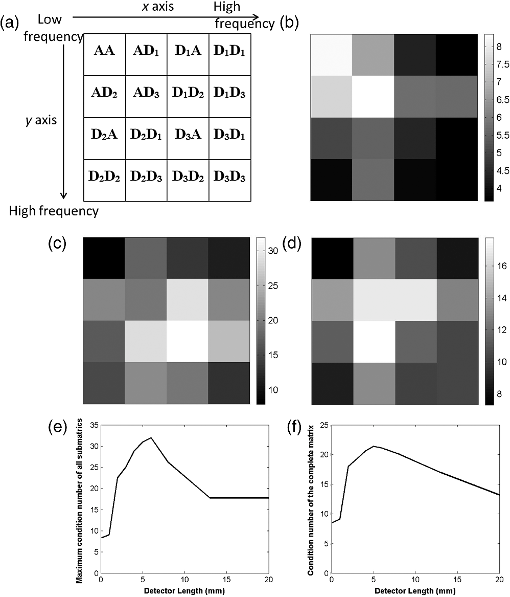

To verify the nonmonotonic dependency of the condition number on detector length, the condition number of the model matrix $\mathbf{M}$ was calculated directly for various detector lengths. The result shown in Fig. 2(f) reveals a behavior similar to that observed by the WP-based analysis. For the calculation of the condition number, the MATLAB built-in function “condest” was used, which is based on the 1-norm condition estimator of Hager.³² This algorithm gives an estimate for the condition number without performing SVD, enabling its practical execution despite the size of the model matrix. Nonetheless, the condition-number calculations required the use of a PC workstation with 160 GB RAM, whereas the SVD performed on the reduced matrices ${\overline{\mathbf{M}}}_w^i$ for Figs. 2(b)–2(e) was executed on a standard desktop with a RAM of only 16 GB.

The advantage of GWP-IMMI-FAD is that it not only enables one to find the frequency bands most susceptible to noise in the reconstruction, but also enables the identification of their spatial patterns. This may be achieved by visualizing the rows in ${\mathbf{V}}^i$ corresponding to the minimum singular values in each frequency band. In contrast, applying SVD on the model matrix $\mathbf{M}$, when computationally feasible, can enable the identification of spatial patterns, but without restriction to specific frequency bands. Figure 3(a) shows the image generated from the row of ${\mathbf{V}}^i$ that corresponds to the smallest singular value in the frequency band for which the highest condition number was obtained in the case of a 6 mm detector. The figure shows that the highest susceptibility to noise is obtained in the periphery of the image. To verify this result, we simulate the signal of spherical source with a diameter of $200\mu \mathrm{m}$ at the top-left corner of the image, as illustrated in Fig. 3(b). Figure 3(c) shows the detected signals for a point detector and detectors with lengths of 6 and 20 mm, whereas Fig. 3(d) shows their frequency content. Indeed, the figures reveal that there is a more substantial loss of high-frequency data in the signal detected by the 6 mm as compared to the one detected by the 20 mm detector. We note that the signals presented in Figs. 3(c) and 3(d) were calculated using the analytical solutions of Ref. 28 and were not based on the model matrices.

Fig. 3

(a) The image generated by the row in ${\mathbf{V}}^i$, which corresponds to the minimum singular value in all the matrices ${\overline{\mathbf{M}}}_w^i$ calculated with a detector length of 6 mm. The result corresponds to the image for which reconstruction is expected to be most unstable. (b) An illustration of a spherical source with a radius of $200\mu \mathrm{m}$ positioned at the location identified in the previous figure panel. (c) The signals detected from the sphere by detectors of various lengths and (d) their corresponding frequency content.

In order to further demonstrate the validity of the results obtained by GWP-IMMI-FAD, object images were generated by a random process similar to the one used in Ref. 18. The images were reconstructed via TSVD with GWP-IMMI-FAD with several values of $\alpha$ in Eq. (16). Each image consisted of nine smooth spheres (indexed by $i$ for $i=1,\dots ,9$) with random origins, radii, and absorbed optical energy densities, denoted by (${\underline{x}}_i$, ${\underline{y}}_i$), ${\underline{R}}_i$, and ${\underline{A}}_i$, respectively. A representative image is provided in Fig. 4(a). We generated 100 random images, whose statistics are listed in Table 1. The model matrix was built by IMMI-FAD (Ref. 21) described in Eqs. (1)–(3) and used to generate all the synthetic projection data. The mean of Gaussian white noise set in the projection data is 0, while the standard deviation (STD) is 2% of the maximum magnitude of the projection data. The statistical assessments of reconstruction performance with different regularization parameters are shown in Figs. 4(b)–4(d). The quality of the reconstructed images was quantified by calculating the structural similarity (SSIM) and root mean square deviation (RMSD) between them and the originating images, as well as bias-variance analysis, as follows:³³

Eq. (19)

$$\mathrm{SSIM}(x,y)=\frac{(2{\mu }_x{\mu }_y+C_1)(2{\sigma }_{xy}+C_2)}{({\mu }_x^2+{\mu }_y^2+C_1)({\sigma }_x^2+{\sigma }_y^2+C_2)},$$

where $x$ and $y$ represent the originating and reconstructed images, ${\mu }_x$ and ${\mu }_y$ are the corresponding means, ${\sigma }_x^2$ and ${\sigma }_y^2$ are the corresponding variances, $C_1$ and $C_2$ are small positive constant, and ${\sigma }_{xy}$ is the covariance between the images. The values of SSIM can range from 0 to 1, where higher values correspond to a higher degree of similarity between the images. RMSD is expressed by

Eq. (20)

$$\mathrm{RMSD}=\sqrt{\frac{1}{N}\sum _{i=1}^N{(x_i-y_i)}^2},$$

where $x_i$ and $y_i$ are the pixel values of the originating and reconstructed image, and $N$ is the number of pixels.

Fig. 4

(a) Schematic illustration of a random object function, (b) mean SSIM of random objects with different detector lengths and regularization parameters, (c) mean RMSD of random objects with different detector lengths and regularization parameters, (d) bias-variance curve of the reconstructions with different detector lengths (point detector and flat detector with lengths of 1, 2, 3, 4, 5, 6, 8, 13, and 20 mm) and $\alpha$ (0, 0.05, and 0.1). For all detector lengths, $\alpha =0$ (no regularization) gave the highest bias and variance. In terms of both bias and variance, a detector length of 4 mm gives the worst results.

Table 1

Parameters of the random numerical phantoms.

Index	(x̲i, y̲i)		R̲i		A̲i
	Mean (mm)	STD (mm)	Mean (mm)	STD (mm)	Mean (a.u.)	STD (a.u.)
1	(0.001, $-0.001$)	(0.028, 0.028)	0.915	0.031	0.301	0.113
2	(0.002, $-0.005$)	(0.028, 0.029)	0.752	0.028	0.134	0.115
3	($-0.243$, $-0.396$)	(0.028, 0.031)	0.119	0.028	0.472	0.117
4	(0.152, $-0.499$)	(0.029, 0.031)	0.121	0.029	0.478	0.114
5	($-0.395$, $-0.005$)	(0.029, 0.028)	0.251	0.026	0.252	0.111
6	(0.197, 0.055)	(0.029, 0.030)	0.247	0.032	0.269	0.116
7	($-0.892$, $-0.898$)	(0.026, 0.033)	0.097	0.034	0.962	0.113
8	($-0.858$, 0.902)	(0.031, 0.028)	0.079	0.022	0.971	0.105
9	(0.817, 0.807)	(0.023, 0.028)	0.079	0.024	0.980	0.123

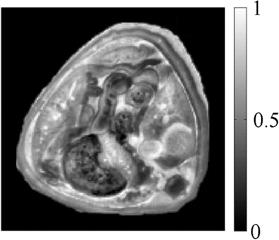
For the calculation of the variance and bias, for each of the random phantom, reconstruction was performed for $M=100$ different additive noise signals generated from a Gaussian distribution with a zero mean and STD of 2% of the maximum projection data. For each pixel, the variance and bias were calculated accordingly.

Eq. (21)

$${\mathrm{Var}}_i=\frac{1}{M}\sum _{j=1}^M{(y_{i,j}-\frac{1}{M}\sum _{j=1}^M{y}_{i,j})}^2,$$

Eq. (22)

$${\mathrm{Bias}}_i=\frac{1}{M}\sum _{j=1}^M{y}_{i,j}-x_i,$$

where $x_i$ and $y_i$ represent the values of the $i^{\prime }$th pixel in the originating and reconstructed image, respectively, $i$ is the pixel index, and $j=1\dots M$ is the index of the added noise signal. The results for the variance and bias are averaged over all pixels and are presented in Fig. 4(d) with different detector lengths (point detector and flat detector with lengths of 1, 2, 3, 4, 5, 6, 8, 13, and 20 mm) and $\alpha$ (0, 0.05, and 0.1).

4.2.

Image Reconstruction for Numerically Generated Data

A numerical study was performed for full- and limited-view scenarios to analyze the imaging performance based on the following reconstruction schemes: BP,⁵ IMMI,¹⁶ IMMI-FAD,²¹ and the proposed GWP-IMMI-FAD. All reconstructed images were normalized. A realistic image of a mouse cross-section, shown in Fig. 5, was used as the originating image, whereas detection was performed over a circle surrounding the image. The size of the originating image was $2\mathrm{cm}\times 2\mathrm{cm}$ with $150\times 150\text{pixels}$. We assumed that a line-segment detector with a length of 13 mm was used for detection and the distance of the detector from the origin was 4 cm. The model matrix was also built by IMMI-FAD and used to generate all the synthetic projection data. All reconstructions were performed for exact and noisy projection data. The noisy data were generated by adding to the projection data Gaussian white noise with zero mean and STD equals to 2% of the maximum projection amplitude. In all cases, the angular increment between the transducer positions was held at 1 deg. The reconstructions were performed in MATLAB on a personal computer with an Intel Core i7 2.1 GHz processor and 16 GB of RAM.

Fig. 5

The numerical phantom used as the originating image in the simulations.

In the reconstructions performed with IMMI and IMMI-FAD, the inversion of the model matrix was performed using Tikhonov regularization. The L-curve method was used to find the Tikhonov regularization parameter $\lambda$.³⁴ In the case of GWP-IMMI-FAD, the WP decomposition was performed using the Daubechies 6 mother wavelet with two-level full-tree decomposition for both the model matrix and projection data, and inversion was performed using TSVD. The L-curve method was also used to find the regularization parameter $\alpha$.³⁴ Figure 6 shows the simulation reconstruction results in a complete-view scenario. Figures 6(a)–6(d), respectively, show the reconstructions using BP, IMMI, IMMI-FAD, and GWP-IMMI-FAD. Figure 6(e) shows a one-dimensional slice generated from the reconstructed image taken along the yellow dashed line in Fig. 6(c). The reconstructions of IMMI obtained without accounting for the detector geometry resulted in a reconstructed blurry image as predicted in Ref. 28, whereas both IMMI-FAD and GWP-IMMI-FAD managed to eliminate the blur. The SSIMs between the original image and Figs. 6(a)–6d) are 0.0753, 0.7023, 0.7748, and 0.7780, respectively. The RMSDs between the original image and Figs. 6(a)–6(d) are 0.3860, 0.0961, 0.0357, and 0.0367, respectively. The total run time of building the WP decomposition matrices in advance was $\sim 1.2\mathrm{h}$. TSVD was used in GWP-IMMI-FAD where truncation was performed using $\alpha =0.02$ in Eq. (16). Nine iterations of Eq. (18) were performed in GWP-IMMI-FAD with each iteration lasting 1 s. Thus, after the precalculation of the matrices, GWP-IMMI-FAD required only 10 s, whereas Tikhonov regularized IMMI-FAD required 215 s.

Fig. 6

Reconstructions of the numerical mouse phantom in complete-view noiseless case using (a) BP, (b) IMMI, (c) IMMI-FAD, and (d) GWP-IMMI-FAD. (e) Absorbed energy density profile of original image, reconstructions of IMMI-FAD and GWP-IMMI-FAD along the yellow dashed line in (c).

Figure 7 shows the images reconstructed from the noisy simulation data for the limited-view scenario in which only the projections on the left side of the images were used (180-deg angular coverage). Figures 7(a)–7(d) show the reconstructions of BP, IMMI, IMMI-FAD, and GWP-IMMI-FAD, respectively. For comparison, we show in Fig. 7(e) the reconstruction obtained via WP-IMMI-FAD with local thresholding [Eq. (13)] and the same value of $\alpha$ as the one used in Fig. 7(d). Figure 7(f) shows the absorbed energy density profile at the same position in Fig. 7(c) among the original image, reconstructions of IMMI-FAD, and GWP-IMMI-FAD. The SSIMs between the original image and Figs. 7(a)–7(e) are 0.0552, 0.4504, 0.6266, 0.6212, and 0.6090, respectively. The RMSDs between the original image and Figs. 7(a)–7(e) are 0.4114, 0.1858, 0.0833, 0.0792, and 0.0890, respectively. In GWP-IMMI-FAD, TSVD was used in GWP-IMMI-FAD where truncation was performed using $\alpha =0.1$ in Eq. (16). The total run time of building the WP decomposition matrices in advance was $\sim 40\min$. Six iterations of Eq. (18) were used for the proposed method and each iteration required 1 s. Accordingly, the reconstruction time of GWP-IMMI-FAD was only 7 s, whereas IMMI-FAD required 104 s.

Fig. 7

Reconstructions of the numerical mouse phantom from the projections on the left plane alone over 180 deg using (a) BP, (b) IMMI, (c) IMMI-FAD, (d) GWP-IMMI-FAD, and (e) WP-IMMI-FAD. (f) Absorbed energy density profile of original image, reconstructions of IMMI-FAD and GWP-IMMI-FAD along the yellow dashed line in (c).

5.

Experimental Results

In this section, we present the application of GWP-IMMI-FAD on experimental optoacoustic data obtained from imaging microspheres and a mouse brain. The microsphere phantom was made out of transparent agar with a thin layer containing numerous dark polymer microspheres with a diameter of $100\mu \mathrm{m}$, similar to the ones used in Ref. 35. The objects were imaged in the optoacoustic tomography system described in Ref. 21. Briefly, a tunable optical parametric oscillator laser providing $<8\mathrm{ns}$ duration pulses with 30 Hz repetition frequency at the wavelength of 650 nm was used to illuminate the mouse under investigation. The laser’s beam was expanded to $\sim 2\mathrm{cm}$ and split into two beams, allowing a uniform illumination around the imaged object. A 15 MHz cylindrical focused transducer was used to detect the optoacoustic signal with a detection radius of 19.05 mm around the microspheres, while a 7.5 MHz cylindrical focused transducer with a detection radius of 25.9 mm was used for the mouse head. Although acoustic focusing is generally limited by diffraction, it has been shown that this geometry may be approximated by a 2-D model with line-segment detectors.²¹ In order to improve the signal-to-noise ratio of the signals, each projection was obtained by averaging 32 independent measurements. The microspheres reconstruction was set with the size of $2\mathrm{cm}\times 2\mathrm{cm}$ and $200\times 200\text{pixels}$, while the mouse brain reconstruction was set with the size of $1.3\mathrm{cm}\times 1.3\mathrm{cm}$ and $130\times 130\text{pixels}$. All reconstructed images were normalized to their maximum and negative values in the images were set to zero.

Figures 8(a)–8(d), respectively, show the full-view reconstructions of microspheres obtained by BP, IMMI, IMMI-FAD, and GWP-IMMI-FAD. In GWP-IMMI-FAD, TSVD was used where truncation was performed using $\alpha =0.16$ in Eq. (16). Clearly, the reconstruction achieved by GWP-IMMI-FAD was considerably sharper than reconstructions obtained by BP and IMMI and similar to the one obtained by IMMI-FAD. After all the matrices had been precalculated, the reconstruction using GWP-IMMI-FAD with 10 iterations took only 80 s, whereas the IMMI-FAD reconstruction required 1646 s.

Fig. 8

Optoacoustic reconstructions of microsphere from experimental data using (a) BP, (b) IMMI, (c) IMMI-FAD, and (d) GWP-IMMI-FAD.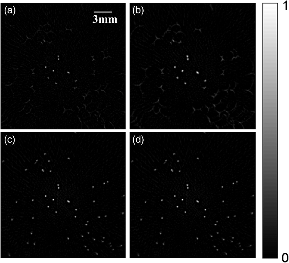

Figures 9(a)–9(d), respectively, show the full-view reconstructions of the mouse brain obtained by BP, IMMI, IMMI-FAD, and GWP-IMMI-FAD. TSVD was used in GWP-IMMI-FAD where truncation was performed using $\alpha =0.08$ in Eq. (16). Clearly, the reconstruction achieved by the model matrices, which included the effect of the line-segment detectors, was sharper than the reconstruction of point detectors. In contrast, the difference between Fig. 9(c) and 9(d) was small and could hardly be detected by visually inspecting the reconstructions. After all the matrices had been precalculated, the reconstruction using GWP-IMMI-FAD with 10 iterations took only 11 s, whereas the IMMI-FAD reconstruction required 197 s.

Fig. 9

Optoacoustic reconstructions of a mouse’s head from experimental data using (a) BP, (b) IMMI, (c) IMMI-FAD, and (d) GWP-IMMI-FAD.

GWP-IMMI-FAD was experimentally demonstrated for limited-view projection data of the mouse brain, in which the angular coverage of the projection data was reduced to 180°. Figures 10(a)–10(c), respectively, show the reconstructions using BP, IMMI, and IMMI-FAD, whereas Fig. 10(d) presents the reconstruction obtained by GWP-IMMI-FAD performed with seven iterations. For TSVD of each matrix, the truncation was performed using $\alpha =0.1$ in Eq. (16). As can be seen in Fig. 10, the use of GWP-IMMI-FAD with TSVD achieved better suppression of the stripe artifact than IMMI-FAD. After the precalculation of the model matrix and reduced matrices, GWP-IMMI-FAD took only 8 s, whereas IMMI-FAD reconstruction required 90 s.

Fig. 10

Optoacoustic reconstructions of a mouse’s head from limited view (180 deg) experimental data obtained using (a) BP, (b) IMMI, (c) IMMI-FAD, and (d) GWP-IMMI-FAD.

6.

Discussion

Model-based optoacoustic reconstruction algorithms offer a promising alternative to conventional BP formulae owing to their ability to be adjusted to arbitrary tomographic geometries. In the case of large-area detectors that are flat over one of their lateral axes, accurate modeling of the detector geometry has shown to improve image fidelity and increase the image resolution. However, the advantage of enhanced images is often overshadowed by the high computational cost model-based inversion incurs, which prevents high-throughput imaging. The case of large-area detectors is especially prohibitive for high imaging rates owing to the substantial increase in matrix size due to the modeling of the detector.

In this paper, we develop GWP-IMMI-FAD, which is the generalization of the WP framework to FADs. Under the WP framework, the image is divided into a set of spatial-frequency bands that are individually reconstructed from only a fraction of the projection data, leading to a set of reduced model matrices. This approach enables the use of TSVD to obtain a regularized inverse matrix to the tomographic problem. In contrast, inversion of the originating model matrix cannot be generally performed using TSVD for high-resolution images owing to the prohibitively large matrix size. Therefore, regularization requires applying iterative optimization algorithms, which are characterized by significantly higher run time. One notable improvement in GWP-IMMI-FAD over the original WP framework, developed for point detector, is the introduction of a global threshold for TSVD. As a result, GWP-IMMI-FAD applies also to cases in which entire spatial-frequency bands in the imaged object are difficult to reconstruct, as seen in the examples presented in Figs. 7(d) and 7(e).

We show that GWP-IMMI-FAD may be used for both system analysis and image reconstruction. In the former case, GWP-IMMI-FAD enables one to calculate the global condition number of each spatial-frequency band and, thus, determine the stability of its reconstruction. Additionally, the use of WPs and SVD enables one to identify which spatial patterns are most difficult to reconstruct and to categorize them based on their spatial frequency. In this work, we used GWP-IMMI-FAD to find the dependency of reconstruction stability on the detector length. In our example, a nonmonotonic relation was obtained in which the global condition number achieved its maximum for a 6 mm long detector. This relation matched well with the condition number of model matrix $\mathbf{M}$ with various detector lengths. Using SVD, we show in Fig. 3 that the reconstruction instability for the 6 mm long detector in the example is most severe for the periphery of the image. Indeed, our analytical analysis revealed that when a small spherical source is positioned at the corner of the image, the signal detected by a 6 mm detector is more low-passed than the one detected by a 20 mm detector.

The result obtained by the analysis of GWP-IMMI-FAD is supposedly inconsistent with the work in Ref. 36, which shows that the amount of smearing created by flat detectors is proportional to the dimensions of their aperture. Based on the analysis in Ref. 36, one might conclude that longer detectors led to stronger attenuation of high frequencies in the projection data and, therefore, that the global condition number should scale with detector length. However, our analysis shows that, in our example in Fig. 3(d), a 6 mm long detector led to stronger attenuation of high frequencies than a 20 mm detector. This supposed contradiction between our results and those of Ref. 36 may be resolved by considering that the analysis in Ref. 36 was performed for a reconstruction algorithm, namely the filtered BP algorithm, which assumes an ideal point detector. Thus, in the context of Ref. 36, any discrepancy between the forward and inverse models would lead to image distortion and possibly smearing. Indeed, although the signal generated by a 20 mm detector is sharper than the one generated by the 6 mm detector, it involves a significantly larger delay when compared to the signal detected by the point detector, as can be seen in Fig. 3(c). Finally, we note that reconstruction formulae exist for the case of infinitely long line detectors,³⁷ whose performance in high-resolution imaging cannot be explained by the analysis given in Ref. 36.

To further validate our conclusions, we compared the reconstructions of randomly generated images obtained with several detector lengths. The reconstruction results revealed a behavior similar to those obtained by the SVD analysis of GWP-IMMI-FAD, namely that starting from a certain detector length, the stability of the reconstruction increases with detector length. The highest reconstruction error in that case was obtained for a detector length of 4 mm. While this value varies from the one obtained via SVD analysis, we note that the randomly generated images represent only a small portion of all the possible images, whereas SVD considers all possible images. Nonetheless, the similar trends obtained in Figs. 2(e)–2(f) and in Figs. 4(b)–4(c) serve as validation to the analysis method developed in this paper. Further validation of this conclusion is obtained from the bias-variance curves in Figs. 4(d), which showed that the variance associated with stability and noise amplification has a nonmonotonic behavior similar to the condition number prediction in Figs. 2(e)–2(f) and the results in Figs. 4(b)–4(c). Finally, we note that the exact values of the condition numbers and reconstruction errors implicitly depend on the resolution specified by the grid on which the image is represented. Increasing the grid resolution is expected to increase the effect of the detector length on the condition number of the matrices describing the system.

The application of GWP-IMMI-FAD for image reconstruction was showcased for simulated and experimental optoacoustic data, wherein both the cases of full- and limited-view tomography were studied. In all examples, the model matrix was too large for applying TSVD directly on it, and Tikhonov regularization was used instead. However, the reduced matrices in the WP decomposition were sufficiently small for performing TSVD. In case of the full-view reconstruction, for both simulation and experimental data, the corresponding reconstruction quality obtained using the proposed GWP-IMMI-FAD was comparable to the one obtained using Tikhonov regularization IMMI-FAD. In case of the limited-view simulation reconstruction, GWP-IMMI-FAD got slightly worse performance than Tikhonov regularization IMMI-FAD did. However, for the limited-view experimental data, GWP-IMMI-FAD achieved better suppression of the stripe artifacts in the reconstruction. In all the examples studied, over an order of magnitude improvement in reconstruction time was achieved by GWP-IMMI-FAD compared to IMMI-FAD.

The performance demonstrated in this work may prove useful for high-throughput optoacoustic imaging studies, which may require the reconstruction of thousands of cross-sectional images. Moreover, the results suggest that the WP framework is not an approach that is restricted to ideal imaging scenarios, but that it could be rather generalized to manage the effects of finite-size aperture and limited-view tomography. Further generalization may be achieved by applying this framework to geometries employing focused detectors as well as to 3-D reconstruction problems, in which a greater need exists for acceleration of model-based reconstruction times. Finally, GWP-IMMI-FAD may be used as a tool for optoacoustic system design. Already in this work, GWP-IMMI-FAD revealed an unknown property of systems with FADs: Beyond a certain detector length, further increments in length may lead not only to stronger optoacoustic signals, but also to more stable reconstructions.