Nonequispaced grid sampling in photoacoustics with a nonuniform fast Fourier transform

Julian Schmid; Thomas Glatz; Behrooz Zabihian; Mengyang Liu; Wolfgang Drexler; Otmar Scherzer

doi:10.1117/1.JBO.21.1.015005

18 January 2016 Nonequispaced grid sampling in photoacoustics with a nonuniform fast Fourier transform

Julian Schmid, Thomas Glatz, Behrooz Zabihian, Mengyang Liu, Wolfgang Drexler, Otmar Scherzer

Author Affiliations +

Journal of Biomedical Optics, Vol. 21, Issue 1, 015005 (January 2016). https://doi.org/10.1117/1.JBO.21.1.015005

Abstract

To obtain the initial pressure from the collected data on a planar sensor arrangement in photoacoustic tomography, there exists an exact analytic frequency-domain reconstruction formula. An efficient realization of this formula needs to cope with the evaluation of the data’s Fourier transform on a nonequispaced mesh. We use the nonuniform fast Fourier transform to handle this issue and show its feasibility in three-dimensional experiments with real and synthetic data. This is done in comparison to the standard approach that uses linear, polynomial, or nearest neighbor interpolation. Moreover, we investigate the effect and the utility of flexible sensor location to make optimal use of a limited number of sensor points. The computational realization is accomplished by the use of a multidimensional nonuniform fast Fourier algorithm, where nonuniform data sampling is performed both in frequency and spatial domain. Examples with synthetic and real data show that both approaches improve image quality.

1. Introduction

Photoacoustic tomography is an emerging imaging technique that combines the contrast of optical absorption with the resolution of ultrasound images (see, for instance, Ref. 1). In experiments, an object is irradiated by a short-pulsed laser beam. Depending on the absorption properties of the material, some of the pulse energy is absorbed and converted into heat. This leads to a thermoelastic expansion, which causes a pressure rise, resulting in an ultrasonic wave called photoacoustic signal. The signal is detected by an array of ultrasound transducers outside the object. Using this signal, the initial pressure is reconstructed, offering a three-dimensional (3-D) image proportional to the amount of absorbed energy at each position. This is the imaging parameter of photoacoustics.

Common measurement setups rely on small ultrasound sensors, which are arranged “uniformly” along simple geometries, such as planes, spheres, or cylinders (see, for instance, Refs. 1 2.3.4.–5). A nonequispaced arrangement of transducers aligned on a spherical array has already been used by Xiang et al.⁶ Here, we investigate photoacoustic reconstructions from ultrasound signals recorded at “not necessarily equispaced” positions on a planar surface. In other words, we use an irregular sensor point arrangement, where sensor points are denser toward the center. This is done in order to maximize image quality, when the number of sensor points is a limiting factor. Our current setup allows to acquire data from 50 sensor points each second. As a consequence, data acquisition of a typical sample requires several minutes. Reducing this acquisition time is a crucial step in advancing photoacoustic tomography toward clinical and preclinical application. This approach can also be seen as new way for dealing with the limited view problem, where deficiencies are caused by a small detection region.

For the planar arrangement of point-like detectors, there exist several approaches for reconstruction, including numerical algorithms based on filtered backprojection formulas and time-reversal algorithms (see, for instance, Refs. 3 and 7 8.–9).

The suggested algorithm in the present work realizes a Fourier inversion formula [see Eq. (1) below] using a fast Fourier transform (FFT) method suitable for nonequispaced grid points and frequencies.¹⁰^–¹² Such methods have been designed for evaluation of Fourier transforms at nonequispaced points in frequency domain, or nonequispaced data points in spatial, respectively, temporal domain. In the present realization introduced in Ref. 13, the prior is called nonequispaced range nonuniform FFT (NER-NUFFT), whereas the latter is called nonequispaced data nonuniform FFT (NED-NUFFT). Both NUFFT methods have proven to achieve high accuracy and simultaneously reach the computational efficiency of conventional FFT computations on regular grids.¹³

For the reconstruction, we propose a novel combination of NED- and NER-NUFFT, which we call NEDNER-NUFFT, based on the following considerations:

1. The discretization of the analytic inversion formula [Eq. (1)] contains evaluations at nonequidistant sample points in frequency domain.
2. In addition, and this comes from the motivation of this paper, we consider evaluation at nonuniform sampling points.

The first issue can be solved by a NER-NUFFT implementation: For two-dimensional (2-D) photoacoustic inversion with “uniformly” placed sensors on a “measurement line,” such an implementation has been considered in Ref. 14. Furthermore, this method was used for biological photoacoustic imaging in Ref. 15. In both papers, the imaging was realized in 2-D due to the use of integrating line detectors.¹⁶^,¹⁷ In this paper, we will analyze the NER-NUFFT in a 3-D imaging setup with point sensors for the first time. The second issue is solved by employing the NED-NUFFT;¹³ thus, the name NEDNER-NUFFT for the combined reconstruction algorithm.

The outline of this work is as follows: In Sec. 2, we outline the basics of the Fourier reconstruction approach by presenting the underlying photoacoustic model. We state the Fourier domain reconstruction formula [Eq. (1)] in a continuous setting. Moreover, we figure out two options for its discretization. We point out the necessity of a fast and accurate algorithm for computing the occurring discrete Fourier transforms (DFTs) with nonuniform sampling points. In Sec. 3, we briefly explain the idea behind the NUFFT. We state the NER-NUFFT (Sec. 3.1) and NED-NUFFT (Sec. 3.2) formulas in the form we need it to realize the reconstruction on a nonequispaced grid. In Sec. 4, we introduce the 3-D experimental setup.

The sections thereafter describe the realized experiments. In Sec. 5, we compare the NER-NUFFT with conventional FFT reconstruction for synthetic data in 3-D. For the real data comparisons, we add a time-reversal reconstruction. Section 6 explains how we choose and implement the nonequispaced sensor placement. In Sec. 7, we turn to the NEDNER-NUFFT in 2-D with simulated data, in order to test different sensor arrangements in an easily controllable environment. In Sec. 8, we interpolate an irregular equisteradian sensor arrangement data from experimentally acquired datasets. We apply our NEDNER-NUFFT approach to the nonuniform data and quantitatively compare the reconstructions to regular grid reconstructions. We conclude with a summary of the results in Sec. 9, where we also discuss the benefits and limitations of the presented methods.

2. Numerical Realization of a Photoacoustic Inversion Formula

Let $U \subset R^{d}$ be an open domain in $R^{d}$ , and $Γ$ a $d - 1$ dimensional hyperplane not intersecting $U$ . Mathematically, photoacoustic imaging consists in solving the operator equation:

Q [f] = {p |}_{Γ \times (0, \infty)},

where

f

is a function with compact support in

U

and

Q [f]

is the trace on

Γ \times (0, \infty)

of the solution of the equation:

\partial_{t t} p - Δ p = 0 in R^{d} \times (0, \infty), p (\cdot, 0) = f (\cdot) in R^{d}, \partial_{t} p (\cdot, 0) = 0 in R^{d} .

In other words, the photoacoustic imaging problem consists in identifying the initial source

f

from measurement data

g = {p |}_{Γ \times (0, \infty)}

.

An explicit inversion formula for $Q$ in terms of the Fourier transforms of $f$ and $g := Q [f]$ has been first formulated by Norton and Linzer¹⁸ and introduced to photoacoustics by Köstli et al.¹⁹ Let $(x, y) \in R^{d - 1} \times R^{+}$ . Assume without loss of generality (by choice of proper basis) that $Γ$ is the hyperplane described by $y = 0$ . Then, the reconstruction reads as follows:

Eq. (1)

F [f] (K) = \frac{2 K_{y}}{κ (K)} F [Q f] [K_{x}, κ (K)],

where

F

denotes the

d

-dimensional Fourier transform:

F [f] (K) := \frac{1}{{(2 π)}^{n / 2}} \int_{R^{d}} e^{- i K \cdot (x, y)} f (x) d x,

and

κ (K) = sign (K_{y}) \sqrt{K_{x}^{2} + K_{y}^{2}}, K = (K_{x}, K_{y}) .

Here, the variables

x

,

K_{x}

are in

R^{d - 1}

, whereas

y

,

K_{y} \in R

.

For the numerical realization, these three steps have to be realized in discrete form. We hereby largely follow the description in Ref. 14. In addition, we give the formula accordingly for the case of measurements taken on nonequispaced grid points.

Let us denote evaluations of a function $ϕ$ at sampling points $(x_{m}, y_{n}) \in {(- X / 2, X / 2)}^{d - 1} \times (0, Y)$ by

Eq. (2)

ϕ_{m, n} := ϕ (x_{m}, y_{n}) .

For convenience, we will modify this notation in case of evaluations on an equispaced Cartesian grid. We define the $d$ -dimensional grid

G_{x} \times G_{y} := {- N_{x} / 2, \dots, N_{x} / 2 - 1}^{d - 1} \times {0, \dots, N_{y} - 1},

and assume our sampling points to be located on

m Δ_{x}

,

n Δ_{y}

, where

(m, n) \in G_{x} \times G_{y},

and write

Eq. (3)

ϕ_{m, n} = ϕ (m Δ_{x}, n Δ_{y}),

where

Δ_{x} := X / N_{x}

, respectively.

Δ_{y} := Y / N_{y}

are the occurring step sizes.

In frequency domain, we have to sample symmetrically with respect to $K_{y}$ . Therefore, we also introduce the interval:

G_{K_{y}} := {- N_{y} / 2, \dots, N_{y} / 2 - 1} .

Since we will have to deal with evaluations that are partially in-grid, partially not necessarily in-grid, we will also use combinations of Eqs. (2) and (3). In this paper, we will make use of discretizations of the source function

f

, the data function

g

and their Fourier transforms

\hat{f}

and

\hat{g}

, respectively.

Let, in the following,

{\hat{f}}_{j, l} = \sum_{(m, n) \in G_{x} \times G_{y}} f_{m, n} e^{- 2 π i (j \cdot m + \ln) / (N_{x}^{d - 1} N_{y})}

denote the

d

-dimensional DFT with respect to space and time. By discretizing formula [Eq. (1)] via Riemann sums, it follows

Eq. (4)

{\hat{f}}_{j, l} \approx \frac{2 l}{κ_{j, l}} \sum_{n \in G_{y}} e^{- 2 π i κ_{j, l} n / N_{y}} \cdot \sum_{m \in G_{x}} e^{- 2 π i (j \cdot m + \ln) / N_{x}^{d - 1}} g_{m, n},

where

κ_{j, l} = s i g n (l) \sqrt{j^{2} + l^{2}}, (j, l) \in G_{x} \times G_{K_{y}} .

This is the formula from Ref. 14.

Remark 1

Note that we use the interval notation for the integer multi-indices for notational convenience. Moreover, we also choose the length of the Fourier transforms to be equal to $N_{x}$ in the first $d - 1$ dimensions, respectively. This could be generalized without changes in practice.

Now, we assume to sample $g$ at $M$ , not necessarily uniform, points $x_{m} \in {(- X / 2, X / 2)}^{d - 1}$ : then,

Eq. (5)

{\hat{f}}_{j, l} \approx \frac{2 l}{κ_{j, l}} \sum_{n \in G_{y}} e^{- 2 π i κ_{j, l} n / N_{y}} \cdot \sum_{m = 1}^{M} \frac{h_{m}}{Δ_{x}^{d - 1}} e^{- 2 π i (j \cdot x_{m}) / M} g_{m, n} .

The term

h_{m}

is a weighting term. It is inversely proportional to the local sampling point density of

x_{m}

on the detector surface and has to fulfill

\sum_{m = 1}^{M} h_{m} = {(N_{x} Δ_{x})}^{d - 1} = X^{d - 1}

. Note that the original formula [Eq. (4)] can be received from [Eq. (5)] by choosing

{x_{m}}

to contain all points on the grid

Δ_{x} G_{x}

.

Equation (5) can be interpreted as follows: once we have computed the Fourier transform of the data and evaluated the Fourier transform at nonequidistant points with respect to the third coordinate, we obtain the (standard, equispaced) Fourier coefficients of $f$ . The image can then be obtained by applying standard FFT techniques.

The straightforward evaluation of the sums on the righthand side of Eq. (5) would lead to a computational complexity of order $N_{y}^{2} \times M^{2}$ . Usually, this is improved by the use of FFT methods, which have the drawback that they need both the data and evaluation grid to be equispaced in each coordinate. This means that if we want to compute Eq. (5) efficiently, we have to interpolate both in domain and frequency space. A simple way of doing that is by using polynomial interpolation. It is used for photoacoustic reconstruction purposes, for instance, in the “k-wave” toolbox for MATLAB.²⁰ Unfortunately, this kind of interpolation seems to be suboptimal for Fourier interpolation with respect to both accuracy and computational costs.¹³^,²¹

A regularized inverse k-space interpolation has already been shown to yield better reconstruction results.²² The superiority of applying the NUFFT, compared to linear interpolation, has been shown theoretically and computationally by Haltmeier et al.¹⁴

3. Nonuniform Fast Fourier Transform

This section is devoted to the brief explanation of the theory and the applicability of the nonuniform Fourier transform, where we explain both the NER-NUFFT (Sec. 3.1) and the NED-NUFFT (Sec. 3.2) in the form (and spatial dimensions) we utilize them afterward.

The NEDNER-NUFFT algorithm used for implementing [Eq. (5)] essentially (up to scaling factors) consists of the following steps:

1. Compute a $d - 1$ dimensional NED-NUFFT in the $x$ -coordinates due to our detector placement.
2. Compute a one-dimensional NER-NUFFT in the $K_{y}$ -coordinate as indicated by the reconstruction formula [Eq. (5)].
3. Compute an equispaced $d$ -dim inverse FFT to obtain a $d$ -dimensional picture of the initial pressure distribution.

Such an algorithm has been introduced in Ref. 11. In contrast to the present approach that is based on Ref. 13, it uses Gaussian bells as window functions. The presented error estimate could be improved in Ref. 12. For a qualitative comparison of the most common available methods, see Ref. 13.

3.1.

Nonequispaced Range Nonuniform Fast Fourier Transform Case

With the NER-NUFFT, it is possible to efficiently evaluate the DFT at nonequispaced positions in frequency domain.

To this end, we introduce the one-dimensional DFT, evaluated at nonequispaced grid points $κ_{l} \in R$ :

Eq. (6)

{\hat{ϕ}}_{l} = \sum_{n \in G_{y}} ϕ_{n} e^{- 2 π i κ_{l} n / N}, l = 1, \dots, M .

In order to find an efficient algorithm for evaluation of Eq. (6), we use a window function $Ψ$ , an oversampling factor $c > 1$ and a parameter $c < α < π (2 c - 1)$ that satisfy:

1. $Ψ$ is continuous inside some finite interval $[- α, α]$ and has its support in this interval and
2. $Ψ$ is positive in the interval $[- π, π]$ .

Then (see Refs. 13 and 14), we have the following representation for the Fourier modes occurring in Eq. (6):

Eq. (7)

e^{- i x θ} = \frac{c}{\sqrt{2 π} Ψ (θ)} \sum_{k \in Z} \hat{Ψ} (x - k / c) e^{- i k θ / c}, | θ | \leq π .

By assumption, both

Ψ

and

\hat{Ψ}

are concentrated around 0. So, we approximate the sum over all

k \in Z

by the sum over the

2 K

integers

k

that are closest to

κ_{l} + k

. By choosing

θ = 2 π n / N - π

and inserting Eq. (7) in Eq. (6), we obtain

Eq. (8)

{\hat{ϕ}}_{l} \approx \sum_{k = - K + 1}^{K} {\hat{Ψ}}_{l, k} \sum_{n \in G_{y}} \frac{ϕ_{n}}{Ψ_{n}} e^{- 2 π i \ln / c N}, l = 1, \dots, M .

Here,

K

denotes the interpolation length and

Eq. (9)

Ψ_{n} := Ψ (2 π n / N_{y} - π), {\hat{Ψ}}_{l, k} := \frac{c}{\sqrt{2 π}} e^{- i π [κ_{l} - (μ_{l, k})]} \hat{Ψ} [κ_{l} - (μ_{l, k})],

where

μ_{l, k}

is the nearest integer (i.e., the nearest equispaced grid point) to

κ_{l} + k

.

The choice of $Ψ$ is made in accordance with the assumptions above, so we need $Ψ$ to have compact support. Furthermore, to make the approximation in Eq. (8) reasonable, its Fourier transform $\hat{Ψ}$ needs to be concentrated as much as possible in $[- K, K]$ . In practice, a common choice for $Ψ$ is the Kaiser–Bessel function, which fulfills the needed conditions, and its Fourier transform is analytically computable.

3.2.

Nonequispaced Data Nonuniform Fast Fourier Transform Case

A second major aim of the present work is to handle data measured at nonequispaced acquisition points $x_{m}$ in an efficient and accurate way. Therefore, we introduce the nonequispaced data, $d - 1$ dimensional DFT

Eq. (10)

{\hat{ϕ}}_{j} = \sum_{m = 1}^{M} ϕ_{m} e^{- 2 π i (j \cdot x_{m}) / N}, j \in G_{x} .

The theory for the NED-NUFFT is largely analogous to the NER-NUFFT,¹³ as described in Sec. 3.1. The representation [Eq. (7)] is here used for each entry of

j

and inserted (with now setting

θ = 2 π n / N

) into formula [Eq. (10)], which leads to

Eq. (11)

{\hat{ϕ}}_{j} \approx \frac{1}{Ψ_{j}} \sum_{m = 1}^{M} \sum_{k \in {- K, \dots, K - 1}^{d - 1}} ϕ_{m} {\hat{Ψ}}_{j, k} \cdot e^{- 2 π i (j \cdot μ_{m, k}) / c M},

where the entries in

μ_{m, k}

are the nearest integers to

x_{m} + k

;. Here, we have used the abbreviations

Ψ_{j, k} := \prod_{i = 1}^{d - 1} Ψ (2 π j / N_{x}), {\hat{Ψ}}_{j, k} := \prod_{i = 1}^{d - 1} (\frac{c}{\sqrt{2 π}}) \hat{Ψ} [{(x_{m})}_{i} - {(μ_{m, k})}_{i}],

for the needed evaluations of

Ψ

and

\hat{Ψ}

.

Further remarks on the implementation of the NED- and NER-NUFFT, as well as a summary about the properties of the Kaiser–Bessel function and its Fourier transform can be found in Refs. 13 and 14.

4. Experimental Setup

Before we turn to the evaluation of the algorithm, we describe the photoacoustic setup. A detailed explanation and characterization of the working principles of our setup can be found in Ref. 23. It consists of a Fabry–Pérot (FP) polymer film sensor for interrogation,²⁴^,²⁵ a 50-Hz pulsed laser source and a subsequent optical parametric oscillator, which emits optical pulses. These pulses have a very narrow bandwidth and can be tuned within the visible and near-infrared range. The optical pulses propagate through an optical fiber. When the light is emitted, it diverges and impinges upon a sample. Some of this light is absorbed and partially converted into heat. This leads to a pressure rise generating a photoacoustic wave, which is then recorded via the FP-sensor head. The sensor head consists of an $\sim 38 μ m$ thick polymer (Parylene C), which is sandwiched between two dichroic dielectric coatings. These dichroic mirrors have a noteworthy transmission characteristic. Light from 600 to 1200 nm can pass the mirrors largely unattenuated, whereas the reflectivity from 1500 to 1650 nm (sensor interrogation band) is about 95%.²³ The acoustic pressure of the incident photoacoustic wave produces a change in the optical thickness of the polymer film. A focused continuous wave laser, operating within the interrogation band, can now determine the change of thickness at the interrogation point via FP interferometry. The frequency response of this specific setup of up to 100 MHz has been analytically predicted, based on a model used in Ref. 25 and experimentally confirmed.²³ There is a linear rolloff reaching zero at 57.9 MHz, with a subsequent rise.

5. Comparison of the Nonequispaced Range Nonuniform Fast Fourier Transform Reconstruction with Fast Fourier Transform and Time Reversal

In this section, several reconstruction methods will be compared for regular grids. This will be done with synthetic data as well as with experimental data. All CPU-based reconstructions are carried out with a workstation PC (Quad Core at 3.6 GHz). All parameters that are not unique to the reconstruction method are left equal.

5.1.

Synthetic Data

For the comparison of different implementations of the FFT-based reconstruction, we conduct a forward simulation of a solid sphere on a $200 \times 200 \times 100$ computational grid, using the “k-wave 1.1” MATLAB library. The maximum intensity projections of the $x y$ and the $x z$ plane of all reconstructions are shown in Fig. 1.

Fig. 1

MIPs in the $x y$ and $x z$ plane of different reconstructions, for a solid sphere. The direct Fourier transform (top) serves as ground truth. $c$ denominates the upsampling factor in the time domain and $k$ the interpolation width of the Kaiser–Bessel function in Eq. (4).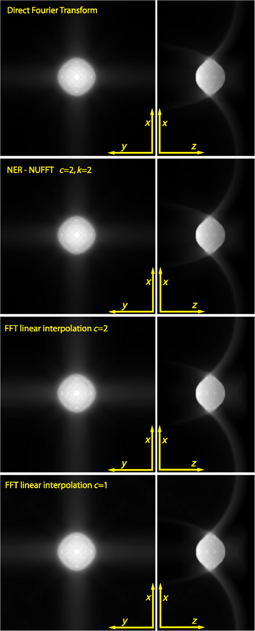

To obtain the closest possible numerical reconstruction of the Fourier-based inversion formula, we directly evaluate the righthand side of Eq. (4), and subsequently invert a 3-D equispaced Fourier transform by applying the conventional 3-D (inverse) FFT. We call this reconstruction “direct FT.” It serves as ground truth for computing the correlation coefficient (Appendix B).

For the NUFFT reconstruction, the temporal frequency oversampling factor in Eq. (8) is set to $c = 2$ and the interpolation length is set to $K = 2$ . In the linear interpolation FFT case, we use both $c = 1$ and $c = 2$ . The FFT reconstruction with $c = 1$ was conducted via the k-wave toolbox, which does not provide oversampling options out of the box. However, the oversampling still can be achieved in a computationally not optimal way by adding zeros at the end of the data term in the time dimension. After reconstruction, the temporal dimension translates into the $z$ axis. In the $x y$ dimension, no oversampling is performed.

The correlation coefficient and the computational time of the methods can be found in Table 1. The errors indicate the superiority of the NUFFT reconstruction in comparison to linear interpolation, with a comparable computational effort (Table 1). The results also show that in the FFT case, an artificial oversampling in the temporal frequency dimension is highly recommended.

Table 1

The first column compares computational times. In the last four columns, the difference to a full correlation with the direct FT reconstruction method is given in %, for the three-dimensional data and the three maximum intensity projections.

	Time	(Correlation-100) in %
	(s)	3-D	xy	xz	yz
NER ( $c = 2$ )	59	0.005	0.0003	0.001	0.001
FFT ( $c = 2$ )	56	3.457	0.54	0.45	0.45
FFT ( $c = 1$ )	53	14.00	0.65	0.81	0.81

5.2.

Experimentally Acquired Data

For an overall qualitative assessment, two datasets, of a 3.5- and a 5-day-old chick embryo, are used.²⁶ This corresponds to the development stages HH21 and HH27 of the Hamburger–Hamilton (HH) criterion.²⁷ The data are sampled with a spatial step size of $60 μ m$ , covering an area of $1.008 \times 1.008 {mm}^{2}$ (3.5 days) and $1.02 \times 1.02 {mm}^{2}$ (5 days) and a time step size of 16 ns, corresponding to a maximum frequency of 31.25 MHz. To avoid aliasing, the signal is low pass filtered to the maximal spatial frequency of 25.3 MHz. A full reconstruction with the NER-NUFFT for the 5-day-old embryo is shown in Fig. 6.

The time reversal reconstruction is performed via the k-wave toolbox. The spatial upsampling factor in the $x$ , $y$ direction is set to 2. For time reversal, this is realized by linearly interpolating the sensor data to a finer grid, whereas for the FFT-based reconstructions, zero padding in the Fourier domain is performed.

The oversampling factor for the FFT reconstructions in the time domain is $c = 2$ . The number of time steps used for the reconstruction covers more than twice the depth range of the visible objects and is 280 for the HH21 and 320 for the HH27 embryo.

In Table 2, a comparison for the computational time is shown. For the NUFFT case, $Ψ$ as defined in Eq. (9) can be precomputed, which roughly halves reconstruction time in subsequent reconstructions using the same discretization, as has been already reported in Ref. 15. Moreover, the computation time improves by a factor of 200 when using FFT-based reconstructions instead of time reversal.

Table 2

Comparison of the computational effort of two chick embryo data sets, with different reconstruction methods.

	Time (s)
Embryo stage27	HH21	HH27
NER-NUFFT ( $k = 2$ , $c = 2$ )	21	24
NER-NUFFT with precomputed $Ψ$	13	14
FFT with linear interpolation ( $c = 2$ )	20	23
Time reversal	7236	7659

The relative Tenenbaum sharpness (Appendix B) for the 3-D data of the 3.5-day-old chick embryo was slightly better for the NER-NUFFT reconstruction (44.2) than for time reversal (43.0) and FFT with linear interpolation (41.1). A comparison of clippings of the maximum intensity projection (MIP) in the $x z$ plane is shown in Fig. 2. The time reversal reconstruction seems smoothed compared to the FFT reconstructions, which is probably a result of the different spatial upsampling modalities.

Fig. 2

The top shows clippings of the MIPs along the $y$ -axis for the two chick embryos. The three reconstruction methods from top to bottom are FFT with linear interpolation, NER-NUFFT, and time reversal. All reconstructions are normalized, so their maximum value is 1. On the bottom graphs, the cumulative signal for each $z$ -axis layer is plotted as a fraction of the corresponding NER-NUFFT layer. While the depth-dependent signal between the time reversal reconstruction and the NER-NUFFT roughly remains the same, for the FFT with linear interpolation, a falloff can be observed. The linear fit suggests a reduction of 10.6% per mm for the 3.5-day-old chick embryo and 13.7% per mm for the 5-day-old chick embryo data.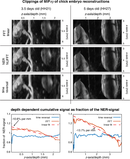

In the bottom graphs of Fig. 2, the cumulative reconstructed signal for each layer is plotted, as fraction of the NER-NUFFT cumulative signal. The additional falloff for the FFT with linear interpolation has been determined by a line fit. For the 3.5-day-old embryo, it was 10.6% per mm and 13.7% per mm for the 5-day-old embryo. While it intuitively makes sense that the $z$ -axis is primarily affected by errors introduced by a suboptimal implementation of Eq. (1), this problem needs further research to be fully understood.

6. Nonequispaced Sensor Placement

The current setups allow data acquisition at just one single sensor point for each laser pulse excitation. Since our laser is operating at 50 Hz, data recording of a typical sample requires several minutes. In an effort to reduce data acqusition time, we try to maximize the image quality for a given number of acquisition points and a given region of interest.

Our newly implemented NEDNER-NUFFT is ideal for dealing with nonequispaced positioned sensors, as error analyses for the NED- and the NER-NUFFT indicate.¹³ This newly gained flexibility of sensor positioning offers many possibilities to enhance the image quality compared to a rectangular grid.

Also any nonequispaced grids that may arise from a specific experimental setup can be efficiently computed via the NEDNER-NUFFT approach.

6.1.

Equiangular and Equisteradian Projections

In this article, we use the NEDNER-NUFFT to tackle the limited view or limited aperture problem, for the case of a limited number of available detectors, which can be placed discretionary on a planar surface. To understand the limited view problem, it is helpful to define a detection region. According to Ref. 28, this is the region which is enclosed by the normal lines from the edges of the sensor. Mathematically speaking, the wavefront propagates on straight lines in the direction of the singularity [Ref. 29, Chapter VIII]. As a consequence, the reconstruction is locally stable if the straight line through the normal to the object boundary passes through the detector surface.³⁰ Therefore, certain edges are invisible to the detector, as depicted in Fig. 3. One approach to overcome this problem experimentally has been made by enclosing the target in a reverberant cavity.³¹ In addition, a lot of effort has been made to enhance reconstruction techniques in order to deal with the limited view problem.²⁸^,³²^–³⁶

Fig. 3

Depiction of the limited view problem. Edges whose normal vectors cannot intersect with the sensor surface are invisible to the sensor. The invisible edges are the coarsely dotted lines. The detection region is marked by a gray background. The finely dotted lines are used to construct the invisible edges. Edges perpendicular to the sensor surface are invisible for a plane sensor.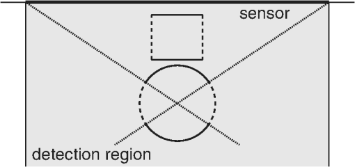

Our approach to deal with this problem is different. It takes into account that in many cases, the limiting factor is the number of sensor points and the limited view is a consequence of this constraint. We use an irregular grid arrangement that is dense close to a center of interest and becomes sparser the further away the sampling points are located. We realize this by means of an equiangular, or equisteradian sensor arrangement, where for a given point of interest, each unit angle or steradian gets assigned one sensor point. This arrangement can also be seen as a mock hemispherical detector.

For the equiangular sensor arrangement, a point of interest is chosen. Each line, connecting a sensor point with the point of interest, encloses a fixed angle to its adjacent line. In this sense, we mimic a circular sensor array on a straight line. The position of the sensor points is pictured on top of the third image in Fig. 4.

Fig. 4

Various reconstructions of a tree phantom (top) with different sensor arrangements. All sensor arrangements are confined to 32 sensor points. The sensor positions are indicated as white rectangles on the top of the images. The second image shows the best (see Fig. 5) equispaced sensor arrangement, with a distance of 13 points between each sensor. The third image shows the NEDNER-NUFFT reconstruction with equiangular arranged sensor positions. The bottom image shows the same sensor arrangement, but all omitted sensor points are polynomially interpolated and afterwards a NER-NUFFT reconstruction was conducted.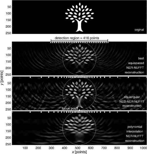

The obvious expansion of an equiangular projection to 3-D is the equisteradian projection. Here, we face a problem analogous to the problem of placing equispaced points on a 3-D sphere and then projecting the points, from the center of the sphere, onto a 2-D plane outside the sphere (the detector plane).

The algorithm used for this projection is explained in detail in Appendix A. Our input variables are the diameter of the detection region, which we define as the diameter of the disc where the sensor points are located, the distance of the center of interest from the sensor plane $r$ and the desired number of acquisition points. In the top left section of Figs. 7 and 8, the sensor arrangements are depicted.

6.2.

Weighting Term

To determine the weighting term $h_{m}$ in [Eq. (5)] for 3-D, we introduce a function that describes the density of equidistant points per unit area $ρ_{p}$ . In our specific case, $ρ_{p}$ describes the density on a sphere around a center of interest. Further we assume that $ρ_{p}$ is spherically symmetric and decreases quadratically with the distance from the center of interest $r : ρ_{p, s} \propto 1 / r^{2}$ . We now define $ρ_{p, m}$ for a plane positioned at distance $r_{0}$ from the center of interest. In this case, $ρ_{p, s} (r)$ attenuates by a factor of $\sin α$ , where $α = \arcsin (r_{0} / r)$ is the angle of incidence. Hence, $ρ_{p, m} \propto r_{0} / r^{3}$ . This yields a weighting term of

h_{m} (r) \propto r^{3} .

Analogously, we can derive

h_{m}

for 2-D:

h_{m} (r) \propto r^{2} .

For the application of this method to the FP setup, it is noteworthy that there is a frequency dependency on sensitivity which itself depends on the angle of incidence. These characteristics have been extensively discussed in Ref. 37.

7. Application of the Nonequispaced Data and Nonequispaced Range Nonuniform Fast Fourier Transform Case with Synthetic Data in Two Dimensions

A tree phantom, designed by Brian Hurshman and licensed under CC BY 3.0,³⁸ is chosen for the 2-D computational experiments on a grid with $x = 1024$ $z = 256$ points. A forward simulation is conducted via k-wave 1.1.²⁰ The forward simulation of the k-wave toolbox is based on a first order k-space model. A perfectly matched layer of 64 grid points is added. Also, white noise is added to obtain an signal to noise ratio of 30 dB.

In Fig. 4, our computational phantom is shown at the top. For each reconstruction, a subset of 32 out of the 1024 possible sensor positions was chosen. In Fig. 4, their positions are marked at the top of each reconstructed image. For the equispaced sensor arrangements, we let the distance between two adjacent sensor points sweep from 1 to 32, corresponding to a detection region sweep from 32 to 1024. The sensor points are always centered in the $x$ -axis.

To compare the different reconstruction methods, we use the correlation coefficient and the Tenenbaum sharpness. These quality measures are explained in Appendix B.

We apply the correlation coefficient only within the region of interest marked by the white circle in Fig. 4. The Tenenbaum sharpness was calculated on the smallest rectangle, containing all pixels within the circle. The results are shown in Fig. 5.

Fig. 5

Correlation coefficient and Tenenbaum sharpness for equispaced sensor arrangements with intervals between the sensor points reaching from 1 to 32. The maximum of the correlation coefficient is at 13. The corresponding reconstruction is shown in Fig. 4. The straight lines indicate the results for the equiangular projection.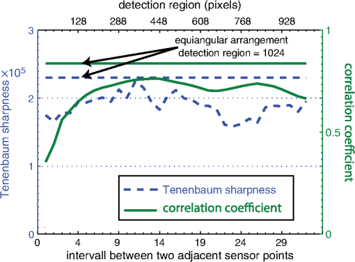

The Tenenbaum sharpness for the equiangular sensor placement is 23001, which is above all values for the equispaced arrangements. The correlation coefficient is 0.913 compared to 0.849, for the best equispaced arrangement. In other words, the equiangular arrangement is 42.3% closer to a full correlation than any equispaced grid.

In Fig. 4, the competing reconstructions are compared. While the crown of the tree is depicted quite well for the equispaced reconstruction, the trunk of the tree is barely visible. This is owed to the limited view of the detection region. As the equispaced interval and the detection region increase, the trunk becomes visible, but at the cost of the crown’s quality. In the equiangular arrangement, a tradeoff between these two effects is achieved. Additionally, the weighting term for the outmost sensors is 17 times the weighting term for the sensor point closest to the middle. This amplifies the occurrence of artifacts, particularly outside the region of interest.

The bottom image in Fig. 4 shows the equiangular sensor arrangement, where the missing sensor points are polynomially interpolated to an equispaced grid and a NER-NUFFT reconstruction is applied afterward. The interpolation is conducted for every time step from our subset to all 1024 sensor points. The correlation coefficient for this outcome was 0.772 while the sharpness measure is 15654. This outcome exemplifies the clear superiority of the NUFFT to conventional FFT reconstruction when dealing with irregular grids.

8. Application of the Nonequispaced Data and Nonequispaced Range Nonuniform Fast Fourier Transform Case with Experimental Data in Three Dimensions

We will now examine if the positive effects of the NEDNER-NUFFT reconstruction with nonequispaced detectors are transferred to 3-D data. For these comparisons, we use the datasets of the two chick embryos already presented in Sec. 5.2. By the use of polynomial interpolation for each time step, we map this data to discretionarily placed points on the acquisition plane. Thus, sensor data is obtained for regular and irregular grids with arbitrary step sizes. The sensor positions are indicated by the red dots in Figs. 7 and 8.

This procedure allows us to use a full reconstruction as a ground truth and thus ensures a quantitative quality control via the correlation coefficient (Appendix B). We are also safe from any experimental errors that could be introduced between measurements. A drawback is that we can only interpolate to step sizes $≧ 60 μ m$ without loss of information. Therefore, the presented images are always made with rather few sensor points and naturally of a lower quality. However, we want to emphasize that this is a result of our experimental procedure.

For all comparison reconstructions, the NEDNER-NUFFT has been used for practical reasons. While the NER-NUFFT cannot deal with nonrectangular grids, it is equivalent to the NEDNER-NUFFT for rectangular regular grids. Using the NEDNER-NUFFT, the spacing of the computational grid can be chosen freely. It corresponds to the width of the Kaiser–Bessel function for interpolation [see Eq. (11)]. If the computational grid is much finer than the local sensor point density, a strong signal close to the sensor surface will produce high intensity spots with an intensity distribution according to the Kaiser–Bessel function, instead of a homogeneous area. Making the computational grid coarser than the sensor point density produces a more blurry reconstruction with a reduced lateral resolution. The computational grid therefore is chosen as fine as possible without reducing the lateral resolution.

We use the two chick embryo datasets to extract the irregular sensor data via layerwise polynomial interpolation. A clipping of the $MIP x z$ of reconstruction of both chick embryos is shown in Fig. 2. A full NER-NUFFT reconstruction of the 5-day-old chick embryo is shown in Fig. 6. For the comparisons, we define a region of interest (ROI) in the form of a cylinder with a height to diameter ratio of 8:9. The area where the sensor points are located for a given reconstruction will be called the “detection region.” The proportions between the ROI and the detection region are the same for all measurements as depicted in Fig. 8.

Fig. 6

MIPs of a full NER-NUFFT reconstruction of a 5-day-old chick embryo (HH27), cropped along the $y$ -axis. Two cylindrical ROIs are indicated, each by a circle and two rectangles. ROI 1 is discussed in Fig. 8 and ROI 2 in Fig. 7. For ROI 1, the focus point for the equisteradian arrangement is shown and the detection region, which marks the area where sensor points are located. The distance $r$ of the “focus point” from the plane governs the size of the detection region and the ROI, according to the proportions shown. Within the detection region, all sensor points occupy the same steradian from the focus point’s perspective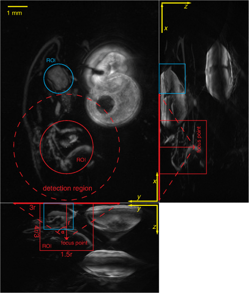

In order to avoid spatial aliasing, the time data have been lowpass filtered with a cutoff frequency according to $F_{cutoff} = c_{sound} / 2 d x$ , where $c_{sound}$ is the sound speed and $d x$ is the step size. In the equisteradian grid, the (locally varying) stepsize $d x$ has been defined as the distance to the nearest neighboring point.

We now conduct a fair comparison between the equisteradian sensor arrangement described in Appendix A and regular grid arrangements for the given ROI. This is done by maximizing image fidelity, while always using (approximately) the same number of sensor points. The comparisons are undertaken for three different ROIs. This is done to show that the advantages of the equisteradian arrangement are not confined to a single case, but rather consistent for different features and volume sizes. All selected ROIs need to have a detection region, that is, fully covered by the underlying data set.

The results are shown in Figs. 2, 7, and 8. The figures are organized in a similar manner and depict different reconstructions via MIPs. On the top left segment, the equisteradian grid arrangement is shown. The top right segment shows the ground truth: a NEDNER-NUFFT reconstruction using all original sensor points that are placed within the detection region. In the segments below, the regular grid reconstructions are shown. On the left, the detection region coincides with the region of interest, on the right, it coincides with the detection region. Figures 7 and 8 also show the sensor point placement. While in the small detection region, the reconstructions have a good resolution, edges are blurred and certain features are invisible. As the detection region increases, these features appear, at the cost of reduced overall resolution. The equisteradian grid arrangement has a rather high resolution toward the center, while still displaying the mentioned features.

Fig. 7

Comparisons of different reconstructions for an ROI, (marked blue in Fig. 6) with roughly 360 sensor points. All reconstructions are presented in the form of MIPs. The top right shows the ground truth, the top left the equisteradian sensor arrangement. Below them, the reconstructions of the regular grids for the largest and the smallest detection region are depicted. On the bottom, the correlation coefficient for different regular grids is shown for the three MIPs and the 3-D data.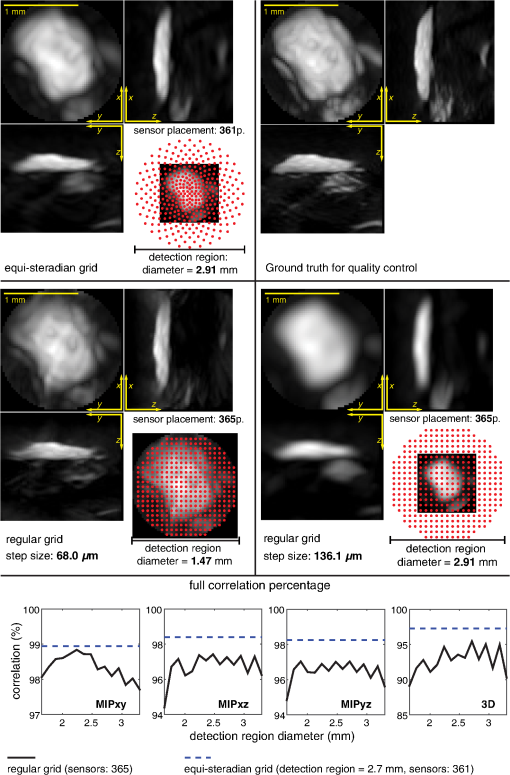

Fig. 8

Comparisons of different reconstructions for an ROI, (marked as red in Fig. 6) with roughly 870 sensor points. All reconstructions have been cropped to the cylindrical ROI. Three MIPs are shown for every reconstruction. The sensor placement is indicated by red dots, which overlay the $MIP x y$ on the bottom right of the dedicated segment. The three bottom segments show regularly arranged sensor points. The detection region diameter (DRD) for the three bottom segments is 2.7, 4, and 5.4 mm while the number of sensor points always remains 869. Certain features (red circle) are not visible for the small detection regions, due to the limited view problem. As the detection region becomes larger, these features start to appear, at the cost of overall resolution. The equisteradian arrangement shown on the top left still shows these features, while maintaining a high resolution. On the top right, a reconstruction with all original points of the detection region is shown. This was used as ground truth. On the top center segment, the correlation coefficient, for different regular grids, is shown.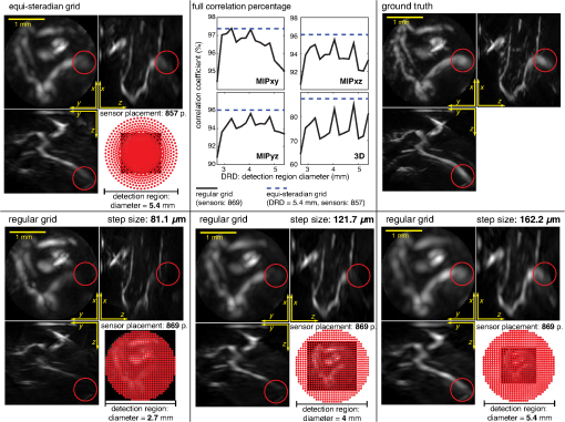

Fig. 9

Reconstruction comparisons of the center region of the 3.5-day-old chick embryo (HH21). The depiction is analog to Fig. 7, without the $MIP y z$ and the sensor placement.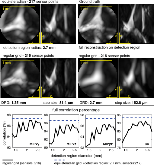

All the above figures contain four graphs, which depict the correlation coefficient for the three MIPs and the volume data. The detection region for the regular grids is increased and shown on the $x$ -axis, while the number of acquisition points stays constant. The computational grid was chosen to be as small as possible but greater than the step size and has been increased in steps of $30 μ m$ in order to have a consistent $μ m / pixel$ spacing in the reconstruction.

The results show that the equisteradian arrangement consistently produces reconstructions that outperform every regular grid arrangement. It provides a good combination of a large detection region and high resolution at the region of interest. This is demonstrated by the juxtaposition of different reconstructions and also confirmed via the correlation coefficient.

9. Conclusions

9.1.

Summary and Results

We computationally implemented a 3-D nonuniform FFT photoacoustic image reconstruction, called NER-NUFFT to efficiently deal with the nonequispaced Fourier transform evaluations arising in the reconstruction formula.

In the computational results, it could be shown that the NER-NUFFT is much closer (more than 100 times in the test piece) to perfect correlation than the FFT reconstruction with linear interpolation.

We then used real datasets for comparison, recorded with a FP-planar sensor setup²³ and included the k-wave time reversal algorithm. Regarding reconstruction time, the results of Haltmeier et al.¹⁴ and Schulze et al.¹⁵ could be confirmed for 3-D, where the FFT with linear interpolation performs similar to NER-NUFFT. Additionally, the NER-NUFFT reconstruction time could be significantly reduced (almost halved), if the values of the interpolation functions $Ψ$ and $\hat{Ψ}$ had already been precomputed for the chosen discretization. The time reversal computation took more than 300 times longer on a CPU, than any FFT-based reconstruction. Concerning image quality, the NER-NUFFT and time reversal reconstruction perform on a very similar level, while the conventional FFT method fails to correctly image the depth-dependent intensity falloff. While this falloff is almost synchronous for time reversal and NER-NUFFT, there was an additional intensity drop of about 10% per mm in the linear interpolation FFT-based reconstruction.

The second application of the NUFFT approach concerned the applicability of irregular grid arrangements, which were new in photoacoustic tomography. In fact, this was done by implementing the NEDNER-NUFFT. Our goal was to maximize image quality in a given region of interest, using a limited number of sensor points. To do this, we developed an equiangular sensor placement for 2-D and an equisteradian placement in 3-D, which assigns one sensor point to each angle/steradian for a given center of interest.

For the 2-D simulations, we showed that this arrangement enhances the image quality for a given region of interest and a confined number of sensor points in comparison to regular grids.

In 3-D, we used the aforementioned chick embryo data and reconstructed with an interpolated subset of the original sensor data. We thus conducted a fair comparison between regular grid arrangements and the equisteradian arrangement with a limited number of sensor points for three ROIs. While the volume of these regions ranged from 1.7 to $13.7 {mm}^{3}$ , the shape always remained a cylinder with a height-to-diameter ratio of $8 ∶ 9$ .

For our ROIs, the correlation of the equisteradian arrangement to the full reconstruction was consistently higher than any regular grid arrangement, using an almost equal number of sensor points.

9.2.

Discussion

For the case of regular sampled grids, the results of Haltmeier et al.¹⁴ were confirmed for 3-D in the synthetic data experiments. The synthetic data results further show the importance of using a zero-pad factor of at least 2 in the time domain, when using FFT-based reconstruction methods. In the case of real data, the main identifiable difference was the additional intensity drop for greater depth of the FFT reconstruction in comparison to the other two methods. The great computational advantage of using FFT-based reconstructions makes it the most suitable method for most cases in a planar sensor geometry setup. There was no detectable difference in the reconstruction quality between the NER-NUFFT and time reversal. From our point of view, the use of the NER-NUFFT therefore seems to be especially useful in the case of high resolution imaging in relatively deep-lying regions.

The NEDNER-NUFFT implementation allowed to efficiently reconstruct data from nonequispaced sensor points. This is used to extend the primary application of a planar sensor surface, recording images over a large area, by the possibility to image a well defined region of interest with a shorter acquisition time. Thus, we designed a sensor mask to better image small regions in larger depths at a fixed number of sensor points, using a design that projects an equispaced hemispherical detector geometry onto a planar sensor surface. For this case, our sensor arrangement produced consistently better reconstructions than any regular grid, because it allowed to maintain a high resolution within our ROI, while still capturing features that could only be detected outside the region of interest. In our test examples, the NEDNER-NUFFT further enhances the image quality in deep regions while maintaining a reasonable computational effort.

In comparison to a real hemispherical detector, there is an increase of acoustic attenuation. This is countered by greater accessibility, scalability, and flexibility on the planar detector. The ROI not necessarily needs to fit into a spherical shape, the size of the region of interest just has an upper bound and the number of acquisition points is limited by the measurement time.

As an outlook, we mention that the case where the field of view is much larger than the imaging depth has not been investigated in this paper. For this case, a similar approach of expanding the field of view by nonequispaced sensor point placement is possible. This could mitigate the image degradation toward the boundaries of the detection region. However, the achievable benefit of such a method would decrease with an increase of the ratio of the detection region area to the detection region boundary and the maximum imaging depth.

Appendices

Appendix A:

Algorithm for Equisteradian Sensor Arrangement

In our algorithm, the diameter of the detection region and the distance of the center of interest from the sensor plane is defined. The number of sensor points $N$ will be rounded to the next convenient value.

Our point of interest is placed at $z = r_{0}$ , centered at a square $x y$ grid. The point of interest is the center of a spherical coordinate system, with the polar angle $θ = 0$ at the $z$ -axis towards the $x y$ -grid.

First, we determine the steradian $Ω$ of the spherical cap from the point of interest that projects onto the acquisition point plane via

Ω = 2 π [1 - \cos (θ_{\max})] .

This leads to a unit steradian

ω = Ω / N

with

N

being the number of sensors one would like to record the signal with. The sphere cap is then subdivided into slices

k

which satisfy the condition:

ω j_{k} = 2 π [\cos (θ_{k - 1}) - \cos (θ_{k})],

where

θ_{1}

encloses exactly one unit steradian

ω

and

j_{k}

has to be a power of two, in order to guarantee some symmetry. The value of

j_{k}

doubles, when

r_{s} > 1.8 \cdot r_{k}

, where

r_{s}

is the chord length between two points on

k

and

r_{k}

is the distance to the closest point on

k - 1

. These values are chosen in order to approximate local equidistance between acquisition points on the sensor surface.

The azimuthal angles for a slice $k$ are calculated according to

ϕ_{i, k} = (2 π i) / j_{k} + π / j_{k} + ϕ_{r},

with

i = 0, \dots, j - 1

, where

ϕ_{r} = ϕ_{j_{k - 1}, k - 1} + (k - 1) 2 π / (j_{k - 1})

stems from the former slice

k - 1

. The sensor points are now placed on the

x y

-plane at the position indicated by the spherical angular coordinates:

(pol, az) = [(θ_{k} + θ_{k + 1}) / 2, ϕ_{i, k}] .

Appendix B:

Quality Measures

In the case where a ground truth image is available, we choose the correlation coefficient $ρ$ , which is a measure of the linear dependence between two images $U_{1}$ and $U_{2}$ . Its range is $[- 1,1]$ . A correlation coefficient close to 1 indicates linear dependence.³⁹ It is defined via the variance $Var (U_{i})$ of each image and the covariance $Cov (U_{1}, U_{2})$ of the two images:

Eq. (12)

ρ (U_{1}, U_{2}) = \frac{Cov (U_{1}, U_{2})}{\sqrt{Var (U_{1}) Var (U_{2})}} .

We decided not to use the widely applied $L^{p}$ distance measure because it is a morphological distance, meaning it defines the distance between two images by the distance between their level sets. Therefore, two identical linearly dependent images can have a correlation coefficient of 1 and still a huge $L^{p}$ distance. This can be dealt with by normalizing the data as in Refs. 28 and 35. We choose the correlation coefficient instead, because in experimentally acquired data, single high intensity artifacts can occur, which would have a disproportionately large effect on the normalized $L^{p}$ distance.

In case of experimentally collected data, there are only a few methods available for the comparison of different reconstruction methods. A possible way for measuring sharpness is obtained from a measure for the high frequency content of the image.⁴⁰ Out of the plethora of published focus functions, we select the Tenenbaum function, because of its robustness to noise:

Eq. (13)

F_{Tenenbaum} = \sum_{x, y} {(g * U_{x, y})}^{2} + {(g^{T} * U_{x, y})}^{2},

with

g

as the Sobel operator:

Eq. (14)

g = (\begin{matrix} - 1 & 0 & 1 \\ - 2 & 0 & 2 \\ - 1 & 0 & 1 \end{matrix}) .

Like the $L^{2}$ norm and unlike the correlation coefficient, the Tenenbaum function is an extensive measure, meaning it increases with image dimensions. Therefore, we normalized it to ${\bar{F}}_{Tenenbaum} = F_{Tenenbaum} / N$ , where $N$ is the number of elements in $U$ .

Acknowledgments

This work is supported by the Medical University of Vienna, the European projects FAMOS (FP7 ICT 317744) and FUN OCT (FP7 HEALTH 201880), Macular Vision Research Foundation (MVRF, USA), Austrian Science Fund (FWF), Project P26687-N25 (Interdisciplinary Coupled Physics Imaging), and the Christian Doppler Society (Christian Doppler Laboratory “Laser development and their application in medicine”). We further want to thank Barbara Maurer and Wolfgang J. Weninger from the Center for Anatomy and Cell Biology at the Medical University of Vienna for providing us with the chick embryos.

References

1.

Photoacoustic Imaging and Spectroscopy, CRC Press, Boca Raton, Florida (2009). Google Scholar

2.

P. Beard, “Biomedical photoacoustic imaging,” Interface Focus, 1 602 –631 (2011). http://dx.doi.org/10.1098/rsfs.2011.0028 Google Scholar

3.

M. Xu and L. V. Wang, “Exact frequency-domain reconstruction for thermoacoustic tomography–I: planar geometry,” IEEE Trans. Med. Imaging, 21 823 –828 (2002). http://dx.doi.org/10.1109/TMI.2002.801172 ITMID4 0278-0062 Google Scholar

4.

M. Xu and L. V. Wang, “Time-domain reconstruction for thermoacoustic tomography in a spherical geometry,” IEEE Trans. Med. Imaging, 21 (7), 814 –822 (2002). http://dx.doi.org/10.1109/TMI.2002.801176 ITMID4 0278-0062 Google Scholar

5.

M. Xu and L. V. Wang, “Analytic explanation of spatial resolution related to bandwidth and detector aperture size in thermoacoustic or photoacoustic reconstruction,” Phys. Rev. E, 67 (5), 0566051 (2003). http://dx.doi.org/10.1103/PhysRevE.67.056605 Google Scholar

6.

L. Xiang et al., “4-D photoacoustic tomography,” Sci. Rep., 3 (2013). http://dx.doi.org/10.1038/srep01113 Google Scholar

7.

P. Kuchment and L. Kunyansky, “Mathematics of thermoacoustic tomography,” Eur. J. Appl. Math., 19 191 –224 (2008). http://dx.doi.org/10.1017/S0956792508007353 0956-7925 Google Scholar

8.

M. Xu and L. V. Wang, “Universal back-projection algorithm for photoacoustic computed tomography,” Phys. Rev. E, 71 (1), (2005). http://dx.doi.org/10.1117/12.589146 Google Scholar

9.

M. Xu and L. V. Wang, “Photoacoustic imaging in biomedicine,” Rev. Sci. Instrum., 77 (4), 041101 (2006). http://dx.doi.org/10.1063/1.2195024 RSINAK 0034-6748 Google Scholar

10.

G. Beylkin, “On the fast Fourier transform of functions with singularities,” Appl. Comput. Harmon. Anal., 2 (4), 363 –381 (1995). http://dx.doi.org/10.1006/acha.1995.1026 ACOHE9 1063-5203 Google Scholar

11.

A. Dutt and V. Rokhlin, “Fast Fourier transforms for nonequispaced data,” SIAM J. Sci. Comput., 14 (6), 1368 –1393 (1993). http://dx.doi.org/10.1137/0914081 SJOCE3 1064-8275 Google Scholar

12.

G. Steidl, “A note on fast Fourier transforms for nonequispaced grids,” Adv. Comput. Math., 9 (3–4), 337 –352 (1998). http://dx.doi.org/10.1023/A:1018901926283 ACMHEX 1019-7168 Google Scholar

13.

K. Fourmont, “Non-equispaced fast Fourier transforms with applications to tomography,” J. Fourier Anal. Appl., 9 (5), 431 –450 (2003). http://dx.doi.org/10.1007/s00041-003-0021-1 Google Scholar

14.

M. Haltmeier, O. Scherzer and G. Zangerl, “A reconstruction algorithm for photoacoustic imaging based on the nonuniform FFT,” IEEE Trans. Med. Imaging, 28 (11), 1727 –1735 (2009). http://dx.doi.org/10.1109/TMI.2009.2022623 ITMID4 0278-0062 Google Scholar

15.

R. Schulze et al., “On the use of frequency-domain reconstruction algorithms for photoacoustic imaging,” J. Biomed. Opt., 16 (8), 086002 (2011). http://dx.doi.org/10.1117/1.3605696 JBOPFO 1083-3668 Google Scholar

16.

P. Burgholzer et al., “Thermoacoustic tomography with integrating area and line detectors,” IEEE Trans. Ultrasonics Ferroelect. Freq. Control, 52 (9), 1577 –1583 (2005). http://dx.doi.org/10.1109/TUFFC.2005.1516030 Google Scholar

17.

G. Paltauf et al., “Photoacoustic tomography with integrating area and line detectors,” Photoacoustic Imaging and Spectroscopy, 251 –263 CRC Press, Boca Raton, Florida (2009). Google Scholar

18.

S. J. Norton and M. Linzer, “Ultrasonic reflectivity imaging in three dimensions: exact inverse scattering solutions for plane, cylindrical and spherical apertures,” IEEE Trans. Biomed. Eng., 28 (2), 202 –220 (1981). http://dx.doi.org/10.1109/TBME.1981.324791 IEBEAX 0018-9294 Google Scholar

19.

K. P. Köstli et al., “Temporal backward projection of optoacoustic pressure transients using Fourier transform methods,” Phys. Med. Biol., 46 1863 –1872 (2001). http://dx.doi.org/10.1088/0031-9155/46/7/309 PHMBA7 0031-9155 Google Scholar

20.

B. E. Treeby and B. T. Cox, “k-wave: MATLAB toolbox for the simulation and reconstruction of photoacoustic wave fields,” J. Biomed. Opt., 15 021314 (2010). http://dx.doi.org/10.1117/1.3360308 JBOPFO 1083-3668 Google Scholar

21.

Y. Xu, D. Feng and L. V. Wang, “Exact frequency-domain reconstrcution for thermoacoustic tomography — I: planar geometry,” IEEE Trans. Med. Imaging, 21 (7), 823 –828 (2002). http://dx.doi.org/10.1109/TMI.2002.801172 ITMID4 0278-0062 Google Scholar

22.

M. Jaeger et al., “Fourier reconstruction in optoacoustic imaging using truncated regularized inverse k-space interpolation,” Inverse Probl., 23 S51 –S63 (2007). http://dx.doi.org/10.1088/0266-5611/23/6/S05 INPEEY 0266-5611 Google Scholar

23.

E. Zhang, J. Laufer and P. Beard, “Backward-mode multiwavelength photoacoustic scanner using a planar Fabry-Perot polymer film ultrasound sensor for high-resolution three-dimensional imaging of biological tissues,” Appl. Opt., 47 561 –577 (2008). http://dx.doi.org/10.1364/AO.47.000561 Google Scholar

24.

P. C. Beard, “Two-dimensional ultrasound receive array using an angle-tuned Fabry-Perot polymer film sensor for transducer field characterization and transmission ultrasound imaging,” IEEE Trans. Ultrasonics Ferroelect. Freq. Control, 52 (6), 1002 –1012 (2005). http://dx.doi.org/10.1109/TUFFC.2005.1504022 Google Scholar

25.

P. C. Beard, F. Perennes and T. N. Mills, “Transduction mechanisms of the Fabry-Perot polymer film sensing concept for wideband ultrasound detection,” IEEE Trans. Ultrasonics Ferroelect. Freq. Control, 46 (6), 1575 –1582 (1999). http://dx.doi.org/10.1109/58.808883 Google Scholar

26.

M. Liu et al., “Dual modality optical coherence and whole-body photoacoustic tomography imaging of chick embryos in multiple development stages,” Biomed. Opt. Express, 5 (9), 3150 –3159 (2014). http://dx.doi.org/10.1364/BOE.5.003150 BOEICL 2156-7085 Google Scholar

27.

V. Hamburger and H. L. Hamilton, “A series of normal stages in the development of the chick embryo,” Dev. Dyn., 195 (4), 231 –272 (1992). http://dx.doi.org/10.1002/aja.1001950404 DEDYEI 1097-0177 Google Scholar

28.

Y. Xu et al., “Reconstructions in limited-view thermoacoustic tomography,” Med. Phys., 31 (4), 724 –733 (2004). http://dx.doi.org/10.1118/1.1644531 MPHYA6 0094-2405 Google Scholar

29.

L. Hörmander, The Analysis of Linear Partial Differential Operators I, 2nd ed.Springer Verlag, New York (2003). Google Scholar

30.

A. K. Louis and E. T. Quinto, “Local tomographic methods in sonar,” Surveys on Solution Methods for Inverse Problems, 147 –154 Springer, Vienna (2000). Google Scholar

31.

B. T. Cox, S. R. Arridge and P. C. Beard, “Photoacoustic tomography with a limited-aperture planar sensor and a reverberant cavity,” Inverse Probl., 23 (6), S95 –S112 (2007). http://dx.doi.org/10.1088/0266-5611/23/6/S08 INPEEY 0266-5611 Google Scholar

32.

M. A. Anastasio et al., “Improving limited-view reconstruction in photoacoustic tomography by incorporating a priori boundary information,” Proc. SPIE, 6856 68561B (2008). http://dx.doi.org/10.1117/12.764178 PSISDG 0277-786X Google Scholar

33.

W. Dan et al., “Influence of limited-view scanning on depth imaging of photoacoustic tomography,” Chin. Phys. B, 21 (1), 014301 (2012). http://dx.doi.org/10.1088/1674-1056/21/1/014301 1674-1056 Google Scholar

34.

J. Frikel and E. T. Quinto, “Artifacts in incomplete data tomography with applications to photoacoustic tomography and sonar,” SIAM J. Appl. Math., 75 (2), 703 –725 (2015). http://dx.doi.org/10.1137/140977709 SMJMAP 0036-1399 Google Scholar

35.

C. Tao and X. Liu, “Reconstruction of high quality photoacoustic tomography with a limited-view scanning,” Opt. Express, 18 (3), 2760 –2766 (2010). http://dx.doi.org/10.1364/OE.18.002760 OPEXFF 1094-4087 Google Scholar

36.

K. Wang et al., “Limited data image reconstruction in optoacoustic tomography by constrained total variation minimization,” Proc. SPIE, 7899 78993U (2011). http://dx.doi.org/10.1117/12.875664 PSISDG 0277-786X Google Scholar

37.

B. T. Cox and P. C. Beard, “The frequency-dependent directivity of a planar Fabry-Perot polymer film ultrasound sensor,” IEEE Trans. Ultrasonics Ferroelect. Freq. Control, 54 (2), 394 –404 (2007). http://dx.doi.org/10.1109/TUFFC.2007.253 Google Scholar

38.

http://thenounproject.com/term/tree/16622/ Google Scholar

39.

Handbook of Mathematical Methods in Imaging, Springer, New York (2011). Google Scholar

40.

F. C. A. Groen, I. T. Young and G. Ligthart, “A comparison of different focus functions for use in autofocus algorithms,” Cytometry, 6 (2), 81 –91 (1985). http://dx.doi.org/10.1002/cyto.990060202 CYTODQ 0196-4763 Google Scholar

Biographies for the authors are not available.

CC BY: © The Authors. Published by SPIE under a Creative Commons Attribution 4.0 Unported License. Distribution or reproduction of this work in whole or in part requires full attribution of the original publication, including its DOI.

Citation Download Citation

Julian Schmid, Thomas Glatz, Behrooz Zabihian, Mengyang Liu, Wolfgang Drexler, and Otmar Scherzer "Nonequispaced grid sampling in photoacoustics with a nonuniform fast Fourier transform," Journal of Biomedical Optics 21(1), 015005 (18 January 2016). https://doi.org/10.1117/1.JBO.21.1.015005

Published: 18 January 2016

Access the abstract

JOURNAL ARTICLE
15 PAGES

DOWNLOAD PAPER SAVE TO MY LIBRARY

GET CITATION

CITATIONS

Cited by 9 scholarly publications.

Explore citations on Lens.org

KEYWORDS

Sensors

Fourier transforms

Photoacoustic spectroscopy

Image quality

Reconstruction algorithms

Image sensors

Data acquisition

1.

Introduction

2.

Numerical Realization of a Photoacoustic Inversion Formula

Eq. (1)

Eq. (2)

Eq. (3)

Eq. (4)

Remark 1

Eq. (5)

3.

Nonuniform Fast Fourier Transform

3.1.

Nonequispaced Range Nonuniform Fast Fourier Transform Case

Eq. (6)

Eq. (7)

Eq. (8)

Eq. (9)

3.2.

Nonequispaced Data Nonuniform Fast Fourier Transform Case

Eq. (10)

Eq. (11)

4.

Experimental Setup

5.

Comparison of the Nonequispaced Range Nonuniform Fast Fourier Transform Reconstruction with Fast Fourier Transform and Time Reversal

5.1.

Synthetic Data

Fig. 1

Table 1

5.2.

Experimentally Acquired Data

Table 2

Fig. 2

6.

Nonequispaced Sensor Placement

6.1.

Equiangular and Equisteradian Projections

Fig. 3

Fig. 4

6.2.

Weighting Term

7.

Application of the Nonequispaced Data and Nonequispaced Range Nonuniform Fast Fourier Transform Case with Synthetic Data in Two Dimensions

Fig. 5

8.

Application of the Nonequispaced Data and Nonequispaced Range Nonuniform Fast Fourier Transform Case with Experimental Data in Three Dimensions

Fig. 6

Fig. 7

Fig. 8

Fig. 9

9.

Conclusions

9.1.

Summary and Results

9.2.

Discussion

Appendices

Appendix A:

Algorithm for Equisteradian Sensor Arrangement

Appendix B:

Quality Measures

Eq. (12)

Eq. (13)

Eq. (14)

Acknowledgments

References

Show All Keywords

Keywords/Phrases

Search In:

Publication Years