|
|
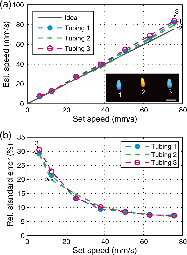
1.IntroductionFlow imaging is a broad and immensely varied field of research. For instance, ultrasound (US) flow imaging is a widely used modality and can be used for relatively low-cost in vivo imaging of arterial functioning1 and of microvasculature.2,3 Although successfully used in many applications, US flow imaging suffers from poor performance at low flow speeds, especially near vessel walls and in small vasculature.4,5 The relatively weak US backscatter of red blood cells (RBCs) in these scenarios is hard to distinguish from the overwhelming tissue backscatter, making flow estimation challenging. Magnetic resonance imaging offers flow imaging using phase contrast and is under investigation for cardiovascular, cerebral, and hepatic flow imaging.6 Although phase contrast magnetic resonance imaging offers a high penetration depth, it remains expensive and time-consuming. Purely optical flow imaging methods, such as orthogonal polarization spectral imaging and optical coherence tomography, can provide more affordable flow imaging.7,8 These techniques allow flow imaging of microvasculature for ophthalmology and dermatology. Although they benefit from high resolution (1 to ), allowing imaging of small capillaries, penetration depth is very limited (1 to 2 mm). Photoacoustic (PA) imaging is a more recent imaging modality and relies on tissue chromophores such as hemoglobin for providing image contrast. In this technique, pressure waves are generated by pulsed or modulated light. This light is absorbed by endogenous or exogenous chromophores, after which a small pressure builds up, which is then released as sound waves.9 The higher optical absorption of RBCs, due to hemoglobin, compared to surroundings makes PA imaging ideal for imaging vascularity, and it can even be used to extract the oxygenation level. Due to their optical absorption, RBCs act as individual PA sources and can consequently be tracked over time, and PA imaging can, therefore, be used for the estimation of blood flow. The advantage of using PA over US for flow imaging is due to low signal amplitudes from surrounding tissues: there is little to no clutter that can affect the flow estimation. Several groups have published work on the use of photoacoustics for the estimation of blood flow; see Ref. 10 for a recent review. Fang et al. used the Doppler shift of CW-modulated photoacoustics to extract velocity information from particle flow.11,10 In a similar approach, Sheinfeld et al. used tone-burst excitation—making a trade-off between spectral and spatial resolution—on particle flow.12 Other techniques include heat-based PA flow estimation, which has been used with blood flow in vitro,13–16 as well as bandwidth broadening with PA microscopy in vivo.17–19 A different method, pulsed photoacoustic flow imaging (pulsed PFI), has a potential advantage over the alternatives in terms of spatial and temporal resolution. Pulsed PFI, like its US counterpart, aims to follow the motion of RBCs over time by tracking an acoustic fingerprint.20 Previous work on pulsed PA flowmetry was performed with high-frequency detection, such as by Brunker and Beard, to estimate particle flow20 and, later, also for estimation of blood flow velocities21 in vitro. The technique has been used in PA microscopy, both in vitro22 and in vivo.23 In addition to using high-frequency detectors, these microscopy studies rely on focused optical excitation. Both optical focusing and high-frequency detection serve to maximize the detectability of the fingerprint signal; however, they also limit the penetration depth, and optical focusing also affects the scanning time of the technique. Both limit clinical applications. High-frequency detection is used for detecting the PA fingerprint of RBCs, since in PA imaging, small absorbers like RBCs—or density variations on a small length scale—generate very high-frequency signals.24,25 This limits the detected fingerprint pressure amplitude even with the typical high-frequency transducers used in microscopy. Additionally, it has been shown that speckle in PA imaging is best visible at high frequencies; at low ultrasonic frequencies, speckle is overshadowed by a constructive boundary pressure wave,26 for instance, in a blood vessel. The latter is one of the reasons PA tomography is devoid of speckle; the fingerprint signal can be regarded as a form of speckle. Nevertheless, the PA frequency response from small absorbing features is also very wide-band, which means the requirement for high-frequency detection is not absolute. In this work, we investigate the feasibility of low-frequency detection for pulsed PFI. To this end, we use a portable and handheld clinical PA system, which integrates a rapid pulsing laser diode and low-frequency array transducer, allowing us to move toward clinical imaging. As such, we approached PFI from the low-frequency detection side instead of lowering the density of absorbers and increasing their size to improve the speckle visibility. We demonstrate the technique using a blood-mimicking phantom using subresolution polyethylene microparticles and show the effects of optical scattering on the performance of the flow estimation. We will conclude with a discussion of the steps required for estimating blood flow using the PA system in vivo. 2.Materials and Methods2.1.Clinical Photoacoustic SystemThe handheld clinical PA system [Fig. 1(a)] is an integrated PA/US probe developed as part of a European Union funded project named FULLPHASE. Based on a design from Ref. 27, the PA/US probe integrates both a 7.5 MHz linear array and an 805 nm pulsed laser module within the housing of a handheld probe. The linear array is adapted from an ESAOTE SL3323 echography probe and is used for the PA detection and US pulse-echo. This array consists of 128 elements with a 7.5 MHz center frequency and a 100% bandwidth. Fig. 1Flow imaging setup: (a) photograph of the clinical PA probe that houses a diode laser on top and ultrasonic detection below and (b) schematic of the alignment to tubing, where is the flow angle. The probe is aligned to have the imaging plane cross the laser illumination. The tubing is looped such that it crosses the imaging plane thrice. 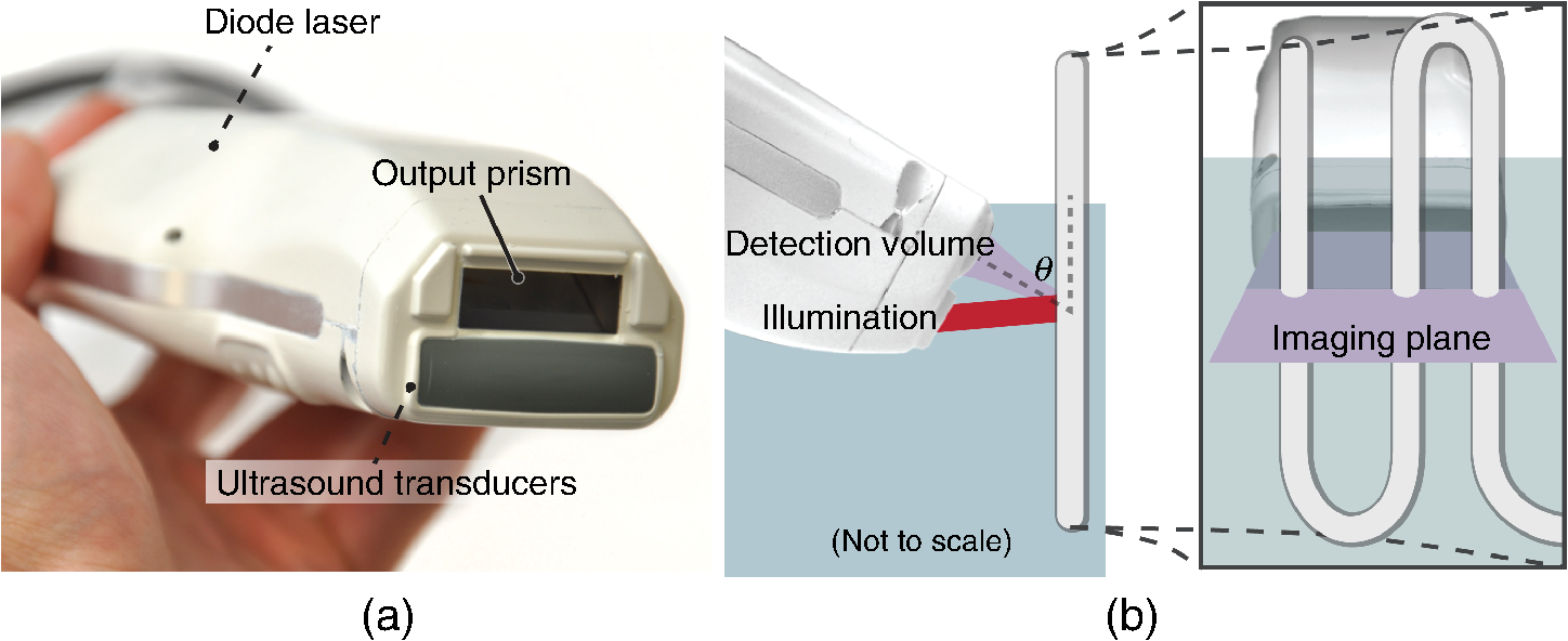 Data acquisition is performed by a MylabOne clinical ultrasound scanner (ESAOTE Europe, Maastricht) at 50 MHz sampling frequency, which transfers prebeamformed data to a laptop. The unprocessed data from the US scanner are then bandpass filtered and reconstructed offline using a Fourier domain algorithm.28 The axial resolution of the system is , and the lateral resolution is .27 The elevational width ranges from , close to the probe, to 1 mm at the acoustic focus, at an axial distance of from the acoustic lens. The relevant elevational thickness for the experiments is 3 mm wide, 5 mm away from the acoustic lens. Laser pulses of 1 mJ and 130 ns are generated by a stack of diode lasers (Osram Opto Semiconductors GmbH, Regensburg, Germany; Quantel, Paris, France). There are four bars stacked vertically, each bar with 64 individual emitters. The diodes are powered by a custom laser driver (Brightloop, Paris, France), which can be triggered by MylabOne. This one laser driver, if triggered, fires all bars simultaneously. The raw beam from the stack is, after collimation, beam-shaped using a diffractive optical element (SILIOS Technologies, Peynier-Rousset, France). A prism is used to change the angle of the beam at the front end of the probe, from which a rectangular beam of 2.2 mm by 17.6 mm () exits the device under an angle of 51 deg. 2.2.Flow PhantomTo validate the setup and the flow estimation, black polyethylene microparticles were used (BKPMS, Cospheric). At 53 to diameter, these particles were smaller than the probe’s resolution but larger and more absorbing than RBCs—which are in their longest dimension—ensuring good detection of individual particles while still demonstrating the principle. Likewise, the concentration was kept to 4% v/v, lower than the 45% v/v of whole blood. The particles were suspended in a 50% v/v glycerol solution to prevent the particles from sedimenting. Polyethylene tubing, with 0.58 and 0.96 mm inner and outer diameters, respectively, was used to model a small artery or vein. The particle suspension was pumped through the tubing using a syringe pump. The expected average flow velocity () was computed from the flow rate () set on the syringe pump. The measurements were started 2 min after initiating the flow; as the particle suspension was viscous, it required some time before the flow was fully developed. The PA probe was placed at an angle to the particle flow [see Fig. 1(b)]. An angle of was used—reducing the internal reflections of PA sound waves within the tubing while still obtaining as long a shift in distance as possible for a certain pulse repetition frequency (PRF). The exact flow angle was measured by moving the probe a distance horizontally using a translation stage. The tubing was then observed moving a distance away from the transducer, from which the flow angle was estimated as . Note that the flow direction determines the sign of the flow velocity: positive and negative for flow toward and away from the transducer, respectively. The probe was positioned 5 mm away such that the illumination from the prism crossed the US detection plane. The polyethylene tubing was looped such that it was visible three times as it crossed the detection plane [see Fig. 1(c)]. Initially, the tubing was placed in a tank filled with water. Later, Intralipid (20% stock) was added to the tank in order to mimic tissue optical scattering and as such improve the realism of the phantom. 2.3.Flow EstimationThe tracking of the PA fingerprint can be performed along the detection time axis by placing the transducer off-normal to a blood vessel of interest. This way, the particles appear to be flowing toward or away from the transducer; therefore, the axial velocity component can be determined by estimating the change in arrival time as shown in Fig. 2(a). A one-dimensional example of a fingerprint signal for the microparticles is shown in Fig. 2(b), where the amplitude is encoded in gray scale along depth. The movement of the particles is visualized by the shift in depth of the fingerprint for subsequent laser pulses. Fig. 2Principle of flow estimation. (a) Side view geometry of estimation principle. Because flow is angled to the transducer axis, any flow will cause a change in arrival time of PA responses from cells or particles. (b) One-dimensional PA measurements of particles for successive laser pulses. (c) Two-dimensional reconstruction of microparticles in tubing, showing the geometry for flow estimation. Flow estimation is performed on axial lines within the reconstruction using a sliding window at positions . See Video 1, MPEG-4, 6 MB [URL: http://dx.doi.org/10.1117/1.JBO.21.2.026004.1]. (d) Mean interpolated cross-correlation for the window indicated in (c), showing a shift in the peak location due to the particle flow. 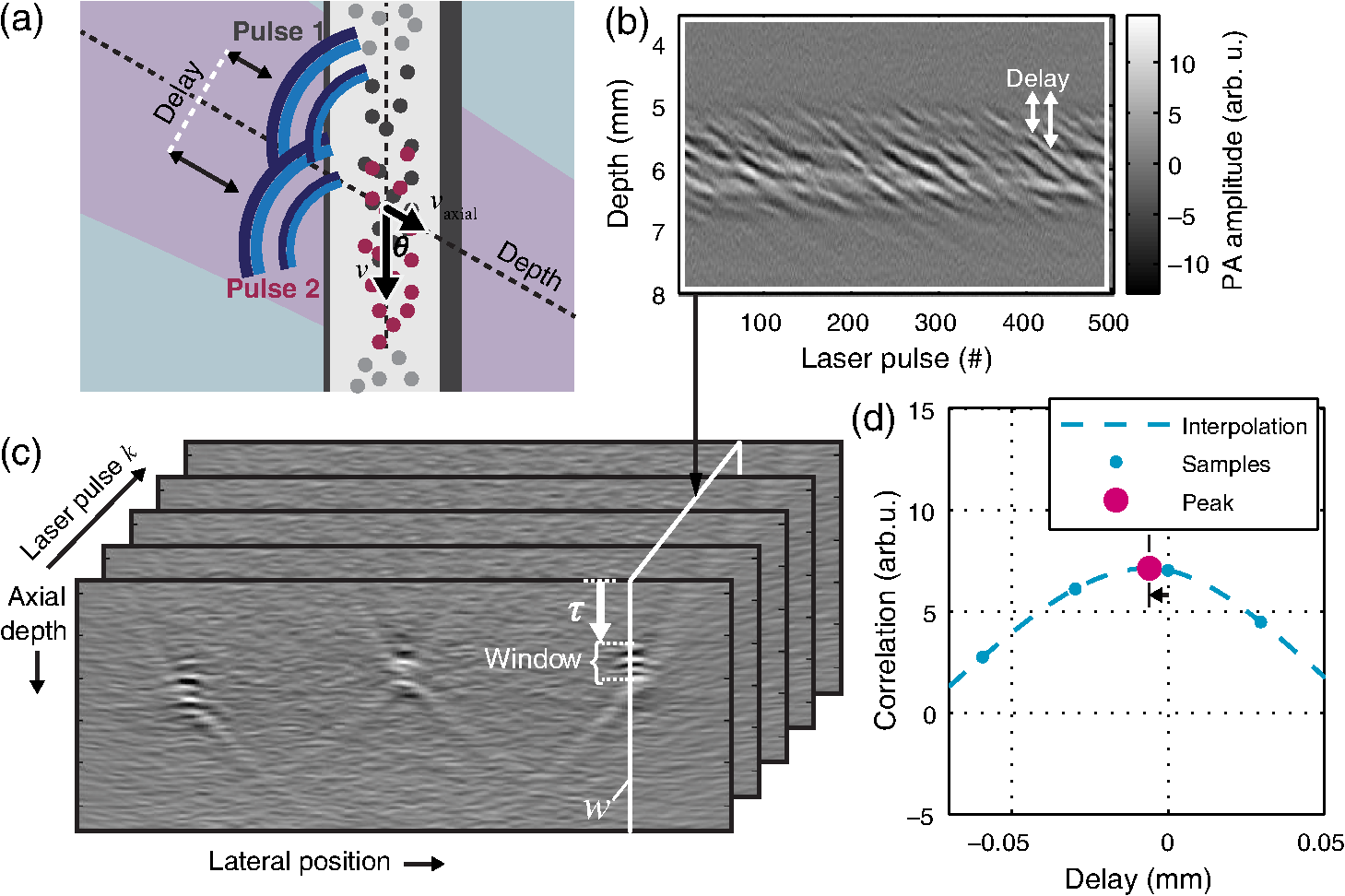 A complete cross-correlation29 was used to estimate flow from axial lines for each lateral position in the PA image [see Fig. 2(c)]. Cross-correlations were performed in a window within , where for each window position , the cross-correlation function was computed between lines and from subsequent pulses and : where is the window length, * denotes the complex conjugate, and is the time-shift index of the cross-correlation. These cross-correlations were averaged, the result of which was spline interpolated at 5 GHz sampling to increase the accuracy of the peak location estimate as shown in Fig. 2(d).The axial flow speed then is , where PRF is the pulse repetition frequency of the laser, the estimated peak location of the cross-correlation for each position of the window, and the speed of sound of the bulk medium. The full flow velocity can be calculated using . PA responses of 500 light pulses were collected with a PRF of 1 kHz, from which the flow was estimated in a window of 10 samples. This window was positioned at depths from 3 to 8 mm for each recorded sample. The pixel size is at 50 MHz, equal to 20 ns, corresponding to at water’s speed of sound. 3.Flow Imaging Results3.1.Validation Using Particles with Water BulkThe clinical PA system is first used for flow imaging with a transparent bulk medium to optimize the signal-to-noise ratio (SNR) and as such validate the technique. The results are presented in Fig. 3, which shows flow images for increasing mean set speeds. Enveloped versions of the PA reconstruction were used to show only flow at regions with a PA amplitude larger than of the maximum (defined here as flow pixels). Fig. 3Flow imaging of microparticles in a transparent bulk medium for a range of speeds. The tubing crosses the imaging plane thrice, flowing up (cross section 2) and down (1 and 3) through the plane. Each image is acquired at a specific pump speed as mentioned in the left column. The ellipse drawn in cross section 1 at represents the physical size of the tubing’s cross section—elliptical due to the imaging angle of 50 deg. 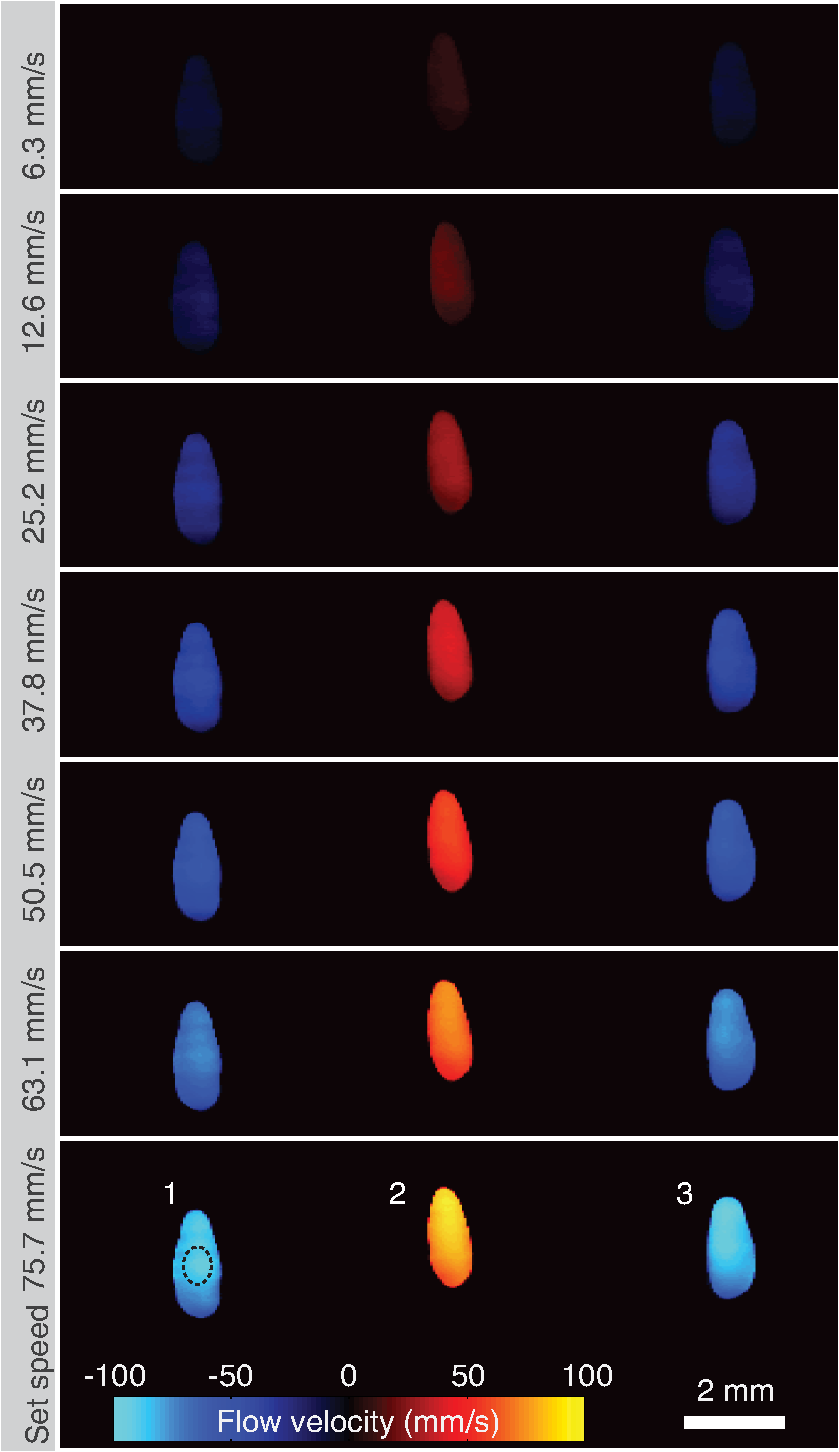 The images show the cross sections of tubing with flows going up (in plane) for number 2, and down for 1 and 3. This is detected as flow toward and away from the transducer, respectively, and expressed as positive and negative flows. Note that the axial positions (the height in the image) are not equal for all three sections. This is a true representation of the flow phantom, in which tubing 2 was somewhat closer to the probe. The absolute mean flow speed per section of tubing is calculated from the relevant flow pixels. The result in Fig. 4(a) shows a good () agreement with the speed set on the syringe pump. In addition, all three tubing sections’ flow speeds are estimated within of each other. Each image shown in Fig. 3 is the average over 10 individual flow images to reduce any random fluctuations in the flow pixels’ velocity. The influence of these fluctuations is determined separately. For each flow pixel, its fluctuations over the 10 individual flow images are computed with the standard error. This results in an error image. The error pixels corresponding to PA pixels are averaged for each section of tubing. This metric, therefore, shows the accuracy of a single pixel of one individual flow image. The result is displayed in Fig. 4(b) as the per-pixel standard error as a percentage of the measured flow speed. The error starts off relatively high at for low speeds of , dropping down to at higher speeds. 3.2.Flow Imaging in a Scattering MediumNext, flow imaging is performed in a scenario where realistic optical scattering reduces the SNR of the detected PA signals. As before, the mean flow speed per tubing section is determined. Figure 5(a) gives the comparison with the set speed, showing a better than 15% agreement between the measurement and the set speed. Rather, the effect of the reduced SNR is mainly visible through the standard error in the flow estimation, as shown in Fig. 5(b). Although it shows a per-pixel standard error that is worse than under nonscattering conditions by a factor of , errors do drop down to at higher flow speeds. Fig. 5Flow quantification performance under realistic optical scattering. For each flow speed, (a) the mean estimated flow speed and (b) the per-pixel error per cross section are evaluated. Compared to optimal (nonscattering) conditions, the mean flow estimation remains accurate, but the standard error is increased due to reduced SNR.  4.Discussion4.1.Flow Imaging PerformancePulsed PFI was successful at both imaging and quantifying flow of 53 to particles. This was true for both a transparent bulk medium and one with realistic optical scattering. Arguably, however, the quantification is more accurate than the imaging resolution, since the axial resolution is somewhat poor (see Fig. 3). While the tubing cross section at a 50 deg intersection angle is 0.76 mm in inner diameter, the imaged axial tubing size is more than twice that value. In part, this is caused by the bandwidth of the transducer, combined with the flow-estimation window size. On the other part, the elevation detection width plays a role, which at width increases the range of axial positions at which the tubing is imaged. The limited resolution likely also prevents imaging of a laminar flow profile, if applicable. The axial resolution can be improved by reducing the flow estimation window size. However, a smaller window size will be at the cost of flow estimation precision. In the flow images with optical scattering, on the other hand, the lateral size is underestimated [see Fig. 5(a), inset], likely because of significantly reduced SNR near the edges of the cross section. In both cases—with and without scattering—there is a small flow gradient visible in the images, with higher flow speeds closer to the probe than farther away. The reason is likely due to a slightly higher density of particles at bigger depth, which would have caused additional friction and slowed down the particles. This higher density of particles would have been caused by a horizontal section of tubing, which supplies the vertical sections seen in the flow images. In this horizontal section, particles would have sedimented slightly, resulting in a somewhat higher density. In the flow estimation, the minimum measureable speed is where the relative error becomes 100%. At optimal SNR—without scattering—this is . With optical scattering, the minimum is . The SNR can be improved by using a higher laser power or more sensitive detectors. The relative error can potentially also be reduced through better flow estimators: in US flow imaging, this can be achieved with Bayesian speckle tracking,30 for example. The maximum measureable speed is determined by the decorrelation of the particle distribution over subsequent laser pulses. This decorrelation can be limited by increasing the PRF of the diode laser, which has an upper pulse rate limit of 10 kHz. The maximum flow speed we measured was , at a PRF of 1 kHz. Therefore, using the probe at its highest PRF will allow flow measurements at speeds higher than . 4.2.Limitations and OutlookThe experiments from this article are performed using microparticles instead of RBCs. We will shortly discuss what would be required—based on this research—for flow imaging of whole blood. RBCs are smaller than the microparticles used here ( versus ) and are denser in whole blood ( versus 4% v/v), but this will not pose a fundamental problem. However, while the overall PA signal might increase with density, the fingerprint visibility will decrease, negatively affecting the SNR of the flow estimation. The increase in density can be addressed by using detectors with narrower elevational focusing, in combination with a higher detector bandwidth. Compared with the current system, using a high-frequency transducer with a 10 MHz bandwidth should sufficiently improve the axial resolution, while not suffering too much from frequency-dependent US attenuation in tissue. Likewise, a 0.5 mm elevational focus should further improve the fingerprint visibility while not limiting the transducer’s depth of field too much. The smaller size of RBCs can be dealt with by increasing the center frequency of the detectors and reducing the pulse length of the laser. In addition, the pulse energy can be increased by adding more laser cavities to the diode laser or by selecting a different laser for further improving the SNR. These changes will serve to improve the fingerprint visibility. Preliminary research shows that flow imaging of whole blood is achievable when implementing most of these improvements. Initial experiments using a 15 MHz transducer (up from 7.5 MHz) and a 4 mJ diode-pumped solid-state laser (up from 1 mJ) with 10 ns long pulses at 500 Hz PRF indicate that flow imaging of whole blood is practically feasible. In an in vivo application of the current clinical PA system, contrast agents could be used to perform the flow imaging, for example, by using fluorophore-filled vesicles. Also, with contrast agents, it holds that PA-based flow imaging would suffer less from sources of clutter than is the case when using US. In general, a realistic comparison of PA and US flow imaging capabilities should be made to test the hypothesis that PA-based flow estimation works better with imaging small vasculature and estimating flow near vessel walls. The flow phantom presented in this article is—when including optical scattering—mainly realistic for PFI, not so much for US flow imaging. Therefore, a specific US/PA flow phantom would have to be developed in order to do the comparison. 5.ConclusionResults of successful pulsed PFI using a clinical handheld PA system were presented. Experiments were performed using microparticles, which were pumped in suspension through tubing, of which cross-sectional flow images were created. The system allowed two-dimensional imaging of multiple tubing sections with opposite flow directions. Quantification performance was evaluated both with the tubing in a transparent medium and with optical scattering that was introduced to mimic tissue . In both cases, flow imaging up to was shown. With optical scattering, the minimum measured speed was ; without scattering, speeds down to can be measured. The estimated mean flow speed agreed within 5% to the pump speed in the transparent medium, and within 15% when optical scattering was introduced. The standard error of the flow estimation suffered somewhat more when reducing the SNR and increased from to 40% (at ) due to optical scattering. In the future, PFI could be used with vesicle-based contrast agents for in vivo flow imaging. Future research should also be directed into flow imaging of whole blood by relying on the availability of high-frequency linear arrays in the 10 to 20 MHz range. In addition, flow estimators developed specifically for PFI could further improve the flow quantification. Flow estimators that rely on specific spectral content or shape of the PA fingerprint, for instance, custom wavelet-based estimators, may improve the estimation considerably. AcknowledgmentsThis research was funded by the European Community’s Seventh Framework Programme (FP7/2007-2013) under Grant Agreement No. 318067 and was partly funded by the European Research Council grant OnQview. ReferencesD. H. Evans, J. A. Jensen and M. B. Nielsen,
“Ultrasonic colour Doppler imaging,”
Interface Focus, 1
(4), 490
–502
(2011). http://dx.doi.org/10.1098/rsfs.2011.0017 JBOPFO 1083-3668 Google Scholar
J. J. Chen et al.,
“A preclinical study to explore vasculature differences between primary and recurrent tumors using ultrasound Doppler imaging,”
Ultrasound Med. Biol., 39
(5), 860
–869
(2013). http://dx.doi.org/10.1016/j.ultrasmedbio.2012.11.005 USMBA3 0301-5629 Google Scholar
E. Filippucci et al.,
“Doppler ultrasound imaging techniques for assessment of synovial inflammation,”
Rep. Med. Imaging, 83
–91
(2013). http://dx.doi.org/10.2147/RMI.S32950 Google Scholar
S. K. Alam and K. J. Parker,
“Implementation issues in ultrasonic flow imaging,”
Ultrasound Med. Biol., 29
(4), 517
–528
(2003). http://dx.doi.org/10.1016/S0301-5629(02)00704-4 USMBA3 0301-5629 Google Scholar
S. Z. Pinter and J. C. Lacefield,
“Detectability of small blood vessels with high-frequency power Doppler and selection of wall filter cut-off velocity for microvascular imaging,”
Ultrasound Med. Biol., 35
(7), 1217
–1228
(2009). http://dx.doi.org/10.1016/j.ultrasmedbio.2009.01.010 USMBA3 0301-5629 Google Scholar
M. Markl et al.,
“4D flow MRI,”
J. Magn. Reson. Imaging, 36
(5), 1015
–1036
(2012). http://dx.doi.org/10.1002/jmri.23632 Google Scholar
W. Groner et al.,
“Orthogonal polarization spectral imaging: a new method for study of the microcirculation,”
Nat. Med., 5
(10), 1209
–1213
(1999). http://dx.doi.org/10.1038/13529 1078-8956 Google Scholar
R. A. Leitgeb et al.,
“Doppler optical coherence tomography,”
Prog. Retin. Eye Res., 41 26
–43
(2014). http://dx.doi.org/10.1016/j.preteyeres.2014.03.004 Google Scholar
L. H. V. Wang and S. Hu,
“Photoacoustic tomography: in vivo imaging from organelles to organs,”
Science, 335
(6075), 1458
–1462
(2012). http://dx.doi.org/10.1126/science.1216210 SCIEAS 0036-8075 Google Scholar
P. J. van den Berg, K. Daoudi and W. Steenbergen,
“Review of photoacoustic flow imaging: its current state and its promises,”
Photoacoustics, 3
(3), 89
–99
(2015). http://dx.doi.org/10.1016/j.pacs.2015.08.001 Google Scholar
H. Fang, K. Maslov and L. V. Wang,
“Photoacoustic Doppler flow measurement in optically scattering media,”
Appl. Phys. Lett., 91
(26), 264103
(2007). http://dx.doi.org/10.1063/1.2825569 APPLAB 0003-6951 Google Scholar
A. Sheinfeld, S. Gilead and A. Eyal,
“Simultaneous spatial and spectral mapping of flow using photoacoustic Doppler measurement,”
J. Biomed. Opt., 15
(6), 066010
(2010). http://dx.doi.org/10.1117/1.3509113 Google Scholar
A. Sheinfeld and A. Eyal,
“Photoacoustic thermal diffusion flowmetry,”
Biomed. Opt. Express, 3
(4), 800
–813
(2012). http://dx.doi.org/10.1364/BOE.3.000800 BOEICL 2156-7085 Google Scholar
L. Wang et al.,
“Ultrasonically encoded photoacoustic flowgraphy in biological tissue,”
Phys. Rev. Lett., 111
(20), 204301
(2013). http://dx.doi.org/10.1103/PhysRevLett.111.204301 PRLTAO 0031-9007 Google Scholar
L. D. Wang et al.,
“Ultrasound-heated photoacoustic flowmetry,”
J. Biomed. Opt., 18
(11), 117003
(2013). http://dx.doi.org/10.1117/1.JBO.18.11.117003 JBOPFO 1083-3668 Google Scholar
R. Y. Zhang et al.,
“In vivo optically encoded photoacoustic flowgraphy,”
Opt. Lett., 39
(13), 3814
–3817
(2014). http://dx.doi.org/10.1364/OL.39.003814 OPLEDP 0146-9592 Google Scholar
B. Ning et al.,
“Simultaneous photoacoustic microscopy of microvascular anatomy, oxygen saturation, and blood flow,”
Opt. Lett., 40
(6), 910
–913
(2015). http://dx.doi.org/10.1364/OL.40.000910 OPLEDP 0146-9592 Google Scholar
S. L. Chen et al.,
“In vivo flow speed measurement of capillaries by photoacoustic correlation spectroscopy,”
Opt. Lett., 36
(20), 4017
–4019
(2011). http://dx.doi.org/10.1364/OL.36.004017 OPLEDP 0146-9592 Google Scholar
J. Yao et al.,
“In vivo photoacoustic imaging of transverse blood flow by using Doppler broadening of bandwidth,”
Opt. Lett., 35
(9), 1419
–1421
(2010). http://dx.doi.org/10.1364/OL.35.001419 OPLEDP 0146-9592 Google Scholar
J. Brunker and P. Beard,
“Pulsed photoacoustic Doppler flowmetry using time-domain cross-correlation: accuracy, resolution and scalability,”
J. Acoust. Soc. Am., 132
(3), 1780
–1791
(2012). http://dx.doi.org/10.1121/1.4739458 JASMAN 0001-4966 Google Scholar
J. Brunker and P. Beard,
“Acoustic resolution photoacoustic Doppler flowmetry: practical considerations for obtaining accurate measurements of blood flow,”
Photonics Plus Ultrasound, 8943 89431K
(2014). http://dx.doi.org/10.1117/12.2039619 Google Scholar
W. Song, W. Liu and H. F. Zhang,
“Laser-scanning Doppler photoacoustic microscopy based on temporal correlation,”
Appl. Phys. Lett., 102
(20), 203501
(2013). http://dx.doi.org/10.1063/1.4807290 APPLAB 0003-6951 Google Scholar
J. J. Yao, K. I. Maslov and L. H. V. Wang,
“In vivo photoacoustic tomography of total blood flow and potential imaging of cancer angiogenesis and hypermetabolism,”
Technol. Cancer Res. Treatment, 11
(4), 301
–307
(2012). http://dx.doi.org/10.7785/tcrt.2012.500278 Google Scholar
G. Diebold, T. Sun and M. Khan,
“Photoacoustic monopole radiation in one, two, and three dimensions,”
Phys. Rev. Lett., 67
(24), 3384
–3387
(1991). http://dx.doi.org/10.1103/PhysRevLett.67.3384 PRLTAO 0031-9007 Google Scholar
E. M. Strohm, E. S. Berndl and M. C. Kolios,
“Probing red blood cell morphology using high-frequency photoacoustics,”
Biophys. J., 105
(1), 59
–67
(2013). http://dx.doi.org/10.1016/j.bpj.2013.05.037 BIOJAU 0006-3495 Google Scholar
Z. J. Guo, Z. Xu and L. H. V. Wang,
“Dependence of photoacoustic speckles on boundary roughness,”
J. Biomed. Opt., 17
(4), 046009
(2012). http://dx.doi.org/10.1117/1.JBO.17.4.046009 JBOPFO 1083-3668 Google Scholar
K. Daoudi et al.,
“Handheld probe integrating laser diode and ultrasound transducer array for ultrasound/photoacoustic dual modality imaging,”
Opt. Express, 22
(21), 26365
–26374
(2014). http://dx.doi.org/10.1364/OE.22.026365 OPEXFF 1094-4087 Google Scholar
M. Jaeger et al.,
“Fourier reconstruction in optoacoustic imaging using truncated regularized inverse k-space interpolation,”
Inverse Prob., 23
(6), S51
–S63
(2007). http://dx.doi.org/10.1088/0266-5611/23/6/S05 INPEEY 0266-5611 Google Scholar
I. A. Hein and W. D. Obrien,
“Current time-domain methods for assessing tissue motion by analysis from reflected ultrasound echoes—a review,”
IEEE Trans. Ultrason. Ferroelectr. Freq. Control, 40
(2), 84
–102
(1993). http://dx.doi.org/10.1109/58.212556 ITUCER 0885-3010 Google Scholar
B. Byram, G. E. Trahey and M. Palmeri,
“Bayesian speckle tracking. Part ii: biased ultrasound displacement estimation,”
IEEE Trans. Ultrason. Ferroelectr. Freq. Control, 60
(1), 144
–157
(2013). http://dx.doi.org/10.1109/TUFFC.2013.2546 ITUCER 0885-3010 Google Scholar
BiographyPim J. van den Berg is a PhD researcher at the University of Twente, the Netherlands. He is working on the European project Fullphase, which aims to develop an affordable and portable ultrasound/photoacoustic (US/PA) system. His main interests are flow imaging using photoacoustics and the application of US/PA imaging for the assessment of rheumatoid arthritis. His interests also include science promotion, having participated in a media push around photoacoustic imaging for the popularization of applied sciences. Khalid Daoudi received his PhD in applied optics on his work on optical-elastography at Institute Langevin, France. Then, he started a postdoctoral position at the BMPI group at University of Twente in the Netherlands. His research focused on methods such as photoacoustics, acousto-optics, and modeling of sound–light tissue interaction. Recently, he joined Radboud University Medical Center in the Netherlands, where he is working on photoacoustic imaging at Medical Ultrasound Imaging Center (MUSIC) group. Wiendelt Steenbergen received his PhD in fluid dynamics at the Eindhoven University of Technology in 1995, after which he joined the University of Twente, Enschede (the Netherlands) as a postdoctorate. In 2000, he was appointed assistant professor in biomedical optics and broadened his scope to low-coherence interferometry and photoacoustic and acousto-optic imaging. In 2010, he became full professor and group leader of the newly formed Biomedical Photonic Imaging group of the University of Twente. |