1.

Introduction

Laser speckle contrast imaging (LSCI) is a simple, noninvasive, low-cost method that allows for the assessment of blood flow and perfusion in near-real time. It has become common place for LSCI and its variations to be used in full-field qualitative visualization of blood flow.^1,2 However, there are numerous experimental challenges, as well as theoretical and practical limitations, that remain unresolved in using LSCI to make quantitative measurements of flow and perfusion.³ Furthermore, for both quantitative and qualitative assessment of blood flows, there are compounding issues such as changes in hematocrit that manifest as changes in bulk blood optical properties that appear identical to relative changes in blood flow. Without a priori knowledge of the scattering and absorption coefficients of the blood, it is impossible to discriminate between changes in flow and changes in blood optical properties.⁴ It is worth noting that the term perfusion is used to describe a relative motion of scatterers in blood vessels. When referring to flow, we describe a volume of scatterers. Because scatterer density has been shown to affect the measured contrast in LSCI,⁴ when we refer to flow and perfusion, we are implying a volume movement of scatterers in time.

In addressing experimental, theoretical, and practical issues in LSCI, it is often difficult to isolate the variables under investigation due to the interdependence of the many experimental parameters. For example, flow, camera integration time, optical arrangement, laser power, and assumed flow model all interact with each other to yield a particular contrast value.^3,5 While phantom flow studies are useful, there are often issues that arise from the experimental design, such as the effects of tubing on the scattering characteristics, unanticipated fluctuations in the flow pattern, clumping of scatterers, and challenges with reproducibility that affect the LSCI results. The challenges associated with phantom flow studies often manifest as noise in the measured contrast value, making it difficult to control single experimental variables. Additionally, computer modeling is useful in understanding the theory behind LSCI, but does not sufficiently address the challenges associated with experimental LSCI.

To address the effects of experimental settings used in LSCI, we utilize an electro-optical system employing a spatial light modulator (SLM) that can faithfully produce LSC images in a highly controlled and reproducible environment.⁶ The system allows for the isolation of single experimental parameters while not varying any others. This optical system permits control of many experimental settings, namely, speckle size, decorrelation behavior of the “scatterers” (and the resulting speckle patterns), the first-order speckle statistics of the speckle patterns (i.e., the intensity probability distribution), the ratio of static to dynamic scatterers, the mathematical relationship between contrast values and the assumed flow model, the camera integration time, and the frame rate. As the objective of this system is to generate dynamic speckle patterns that are statistically (and visually) similar to experimental speckle patterns observed from biological tissue, having the ability to isolate each variable independently means that we can adjust our settings to account for known interdependencies and assess unknown interdependencies between experimental parameters and measured contrast, while having the freedom to address other real experimental variables. For example, the speckle/pixel size ratio has been shown to have an effect on measured contrast value.⁷ Our system allows us to easily adjust the speckle size to ensure that the speckle patterns are sampled spatially in any manner desired by the operator. Once the speckle size is fixed, we can then adjust experimental parameters, such as incident intensity, and assess the effect on measured contrast values as well as the resulting effect on the frequency content of the speckle image.

LSCI is limited by the uncertainty as to the proper flow model used to describe the stochastic behavior of the scattering particles.³ Because of this limitation, the dynamic speckle generated via reflection from the SLM is created using an assumed model. It is worth mentioning that the flow model used in mimicking speckle can be easily adjusted by the user to any model desired, which may serve as a valuable method of comparison between various models of behavior of the scattering particles in the future.

In this work, we focus on adjusting the total intensity of the speckle patterns at the imaging plane and assess the statistics of the resulting speckle patterns. In many practical applications, intensity is addressed as a laser power density incident on a phantom or tissue. When a coherent light source illuminates biological tissue, the photons transmit through, absorb, and scatter within the tissue. Because the amount of energy lost within the tissue can vary greatly between experiments, as well as tissue types in human application, the resulting backscattered light intensity arriving at the imaging plane can have varying levels of intensity. Because of this, describing the incident intensity at a medium does not sufficiently address whether or not the camera is receiving sufficient illumination. We seek to eliminate the variation seen in experimental procedures by addressing the statistical properties of the speckle patterns with varied intensities, as detected by the camera. We address the quantization of camera gray values across a wide range of incident laser power densities, presenting a guideline that can be used when adjusting both camera and laser settings in future applications of LSCI.

2.

Methods and Materials

The optical layout can be seen in Fig. 1. A stabilized 2.5 mW HeNe laser (633 nm) illuminated a $512\times 512$ nematic SLM [Boulder Nonlinear Systems (BNS) XY series, Model-P512] via a beam splitter that returned the scattered light to an 8-bit CMOS camera (Thorlabs, DCC1545M High Resolution USB 2.0 CMOS Camera) with an effective area of $1280\times 1024\text{pixels}$. It is assumed that only the zero-order output pattern from the BNS XY Series nematic SLM is responsible for image reconstruction due to the high zero-order diffraction efficiency of the device.⁸ Additionally, BNS’s high speed addressing scheme is assumed to limit phase drooping and latency, resulting in temporally stable phase modulation.⁸ Before the reflected light was imaged on the CMOS array, the light passed through a $4f$ imaging system with an adjustable aperture stop located in the Fourier plane of the front lens. The lenses comprising the $4f$ imaging system consisted of a 125-mm focal length (FL) achromatic triplet and a 75.0-mm FL achromatic doublet. The effective FL and principal plane of the system were estimated using thin-lens approximations.⁹ The CMOS array was located in the imaging plane, approximately 132 mm from the second lens. The resulting image magnification was roughly 0.5. The aperture stop was placed in the Fourier plane at a distance equal to the FL from each lens. Varying the diameter of the aperture opening changes the minimum speckle size observed on the camera. Reducing the opening of the aperture resulted in larger speckles, while increasing the diameter resulted in smaller speckles.¹⁰ The speckle size, $d_{\mathrm{sp}}$, was estimated by Eq. (1), where $\lambda$ is the illumination wavelength, $v$ is the distance from the principal plane of the lens system to the imaging plane, and $a$ is the diameter of the viewing lens aperture.¹¹

Fig. 1

(a) Optical layout of the LSCI simulating system. The laser was a 2.5-mW stabilized HeNe (633 nm). The FL of $L_1$, $L_2$, and $L_3$ are 75, 125, and 75 mm, respectively. The image magnification equaled $\sim 0.5$. (b) Horizontal view of the imaging arm of the setup. The distance from $L_2$ to $L_3$ was $\sim 300\mathrm{mm}$. The CMOS array was located $\sim 132\mathrm{mm}$ from the back focal plane of $L_3$. The principal plane, ν, was estimated to be $\sim 37.5\mathrm{mm}$ from the CMOS array.

The light passed through a neutral density (ND) filter wheel set to attenuate incoming light, allowing adjustable incident intensity. The beam was then passed through a spatial filter consisting of a $10\times$ microscope objective and a $25\text{-}\mu \mathrm{m}$ pinhole. The beam was then collimated before passing through a $\lambda /2$ plate. The half-wave plate served to orient the polarization of the incoming light in the vertical plane so that the nematic SLM functioned in the phase-only mode. By operating in the phase-only mode, the light backscattered from the SLM was dephased in the same way as if it were scattered from a rough surface or a scattering volume. A polarizer placed in the imaging arm was oriented in the same plane as the incident light. This resulted in observing only a single component of the electromagnetic wave on the CMOS array, thus generating a polarized speckle pattern. Care was taken to ensure negligible ambient light reached the CMOS array.

To generate the speckle patterns from the SLM, a sequence of phase screens, arbitrarily chosen to be 50 frames in length was loaded to the SLM. The phase screens were generated by filling a $512\times 512$ array with randomly generated complex numbers of unit amplitude, with phases uniformly distributed over $[\mathrm{0,2}\pi ]$. For each individual phase screen loaded to the SLM, a predetermined look-up table was used to ensure the phase modulation resulted in a linear relationship between phase distribution $[0,2\pi ]$ and resulting gray values [0, 255]. Thus, light scattered from each individual SLM element was dephased accordingly and the resulting scattered wavefront had an identical phase distribution. The scattered light remained temporally and spatially coherent, allowing for random interference to occur when the scattered light impinged on the CMOS chip of the camera, resulting in a speckle pattern.

The phase screen sequence allowed for controlled temporal decorrelation behavior. By controlling the temporal decorrelation behavior of the phase screens, the temporal decorrelation behavior of the resulting speckle patterns was varied using the copula method.¹² The correlation, $r$, between the speckle patterns was varied over the interval $[1,-1]$. For a specified correlation of $r=1.0$ between multiple phase screens, the resulting phase screens were perfectly correlated, resulting in perfectly correlated sequential speckle patterns. When $r=0$, the phase screens and resulting sequential speckle patterns were completely uncorrelated. Due to the complex symmetric nature of the Fourier transform relating the phase screens to speckle patterns, phase screen realizations of $r\le 0$ result in an uncorrelated speckle pattern. The shape of the decorrelation curve was governed by the rate at which the realization was altered following either a Gaussian or exponential curve, resulting in either Gaussian or Lorentzian decorrelation behavior in the imaged speckle. When generating the phase screens, we invoke the Wiener–Khinchin theorem¹³ to recall that an exponential and a Lorentzian form a Fourier pair, as does a Gaussian and a Gaussian. That is, when the phase screens exhibited a Gaussian decorrelation behavior, the resulting speckle pattern sequence also exhibited Gaussian behavior. When the phase screens exhibited an exponential decorrelation behavior, the speckle sequence exhibited Lorentzian behavior. In the present work, the decorrelation time of the generated speckle frames was arbitrarily chosen to be 17 (fast) and 37 (slow) frames. An example of Gaussian phase screen decorrelation behavior, showing varying decorrelation times, can be seen in Fig. 2. Figure 2 also demonstrates the ability to change the shape of the autocorrelation function between Gaussian and Lorentzian.

Fig. 2

Decorrelation curve for SLM speckle patterns with different correlation behavior exhibiting a Gaussian decorrelation profile. For this example, 50 screens were created to image 50 consecutive speckle patterns. (a) Decorrelation time of 37 frames, (b) Decorrelation time of 17 frames, (c) Demonstration of both Lorentzian and Gaussian decorrelation behaviors showing a Lorentzian autocorrelation function (stars) plotted along with a Gaussian autocorrelation function (dots).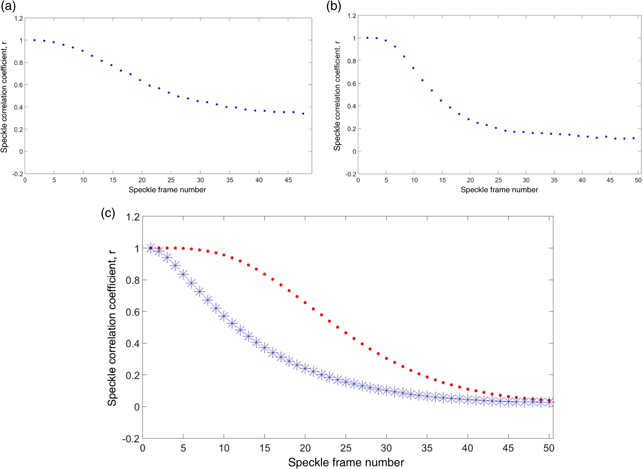

Once the phase screens were generated and loaded to the SLM, each resulting speckle pattern was imaged individually by the CMOS camera. The camera was set to expose each static speckle pattern for 35 ms. An example showing a single phase screen and the resulting imaged speckle pattern can be seen in Fig. 3. Using the imaged speckle patterns generated by the SLM, the first-order statistics of the coherent summation were assessed and described by the intensity probability distribution function (PDF). A comparison of the theoretical and experimental PDF for fully polarized speckle is displayed in Fig. 4. For a polarized speckle pattern, the theoretical PDF is a negative exponential.¹⁰ Figure 4(a) demonstrates the ability to reproduce a single speckle pattern with a negative exponential PDF. In cases where multiple speckle patterns are incoherently summed, the PDF of the resultant speckle pattern is described by a Rayleigh distribution. In practice, such a speckle pattern can also be seen when observing speckle from a volume scatterer, such as tissue, without using a polarizer to isolate a single component of the electromagnetic field. Figure 4(b) shows the system’s ability to reproduce speckle with a Rayleigh PDF, by summing on an intensity basis, multiple individual polarized speckle patterns. The number of speckle patterns that needs to be summed to generate a speckle pattern with a Rayleigh PDF, as in Fig. 4(b), depends upon the decorrelation behavior of the speckle sequence. The lower the correlation between subsequent speckle patterns, the fewer individual patterns need to be summed. In the limiting case, only two speckle patterns are necessary if they are statistically independent from one another.¹⁰

Fig. 3

(a) Phase screen loaded to the SLM. The pixel-phases were evenly distributed and randomly generated between $[0,2\pi ]$. The pixel values are displayed as a psudocolor image with 64 discrete values. (b) The resulting speckle pattern imaged with an 8-bit CMOS camera. The random interference can be seen mapped to gray values between [0, 255], with a value of 255 indicating purely constructive interference, and 0 resulting from destructive interference.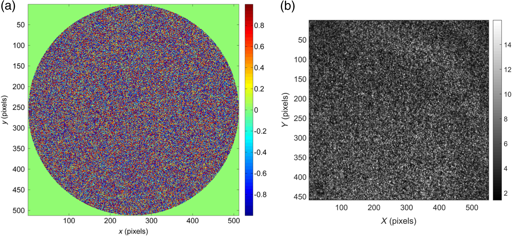

Fig. 4

Intensity PDFs of SLM generated speckle patterns plotted with numerically simulated (theoretically ideal) speckle patterns. (a) Fully developed, polarized intensity PDF showing both experimental (SLM) and theoretical speckle patterns in agreement. (b) Nonpolarized intensity PDF showing both experimental and theoretical results in agreement. It is worth noting that the Rayleigh PDF is often dependent on the scale factor used. For this experiment, the logarithmic scale shows similar linearity to assume an accurate intensity distribution.

The second-order statistics of the interference patterns were analyzed through the power spectral density (PSD) of the imaged speckle pattern. As the calculated PSD can be used to experimentally determine speckle size, we use the calculated speckle size to describe the second-order behavior of the generated speckle patterns. To control the minimum size of the speckle, and thus the second-order characteristics, the camera aperture can be easily adjusted to verify the minimum speckle size in the imaged speckle, the PSD of the imaged speckle was calculated and the diameter of the frequency energy band was measured (in pixels). The size of the minimum imaged speckle was calculated as⁷

Figure 5 shows the variation in speckle size achieved with the SLM-based system. The speckle size for both the experimental and calculated values are displayed relative to the pixel size of the CMOS array. Figure 5(a) shows a single speckle pattern from the SLM and its power spectrum [Fig. 5(b)], which was used to estimate the minimum speckle size in the pattern. Figure 5(c) shows the theoretical speckle size, as calculated with Eq. (1), plotted with the imaged speckle size. For the experiments across varied intensities, the minimum imaged speckle size relative to the CMOS chip pixel size ($5.2\mu \mathrm{m}$) was kept constant at roughly $3.25\text{pixels}/\text{speckle}$.

Fig. 5

(a) SLM generated speckle pattern and (b) SLM generated speckle PSD. The minimum speckle size in this case was 4 pixels. (c) Variation in speckle size plotted as a function of the aperture diameter, with the theoretical curve of Eq. (1) plotted as the solid line. The experimentally sampled speckle size is plotted as blue dots.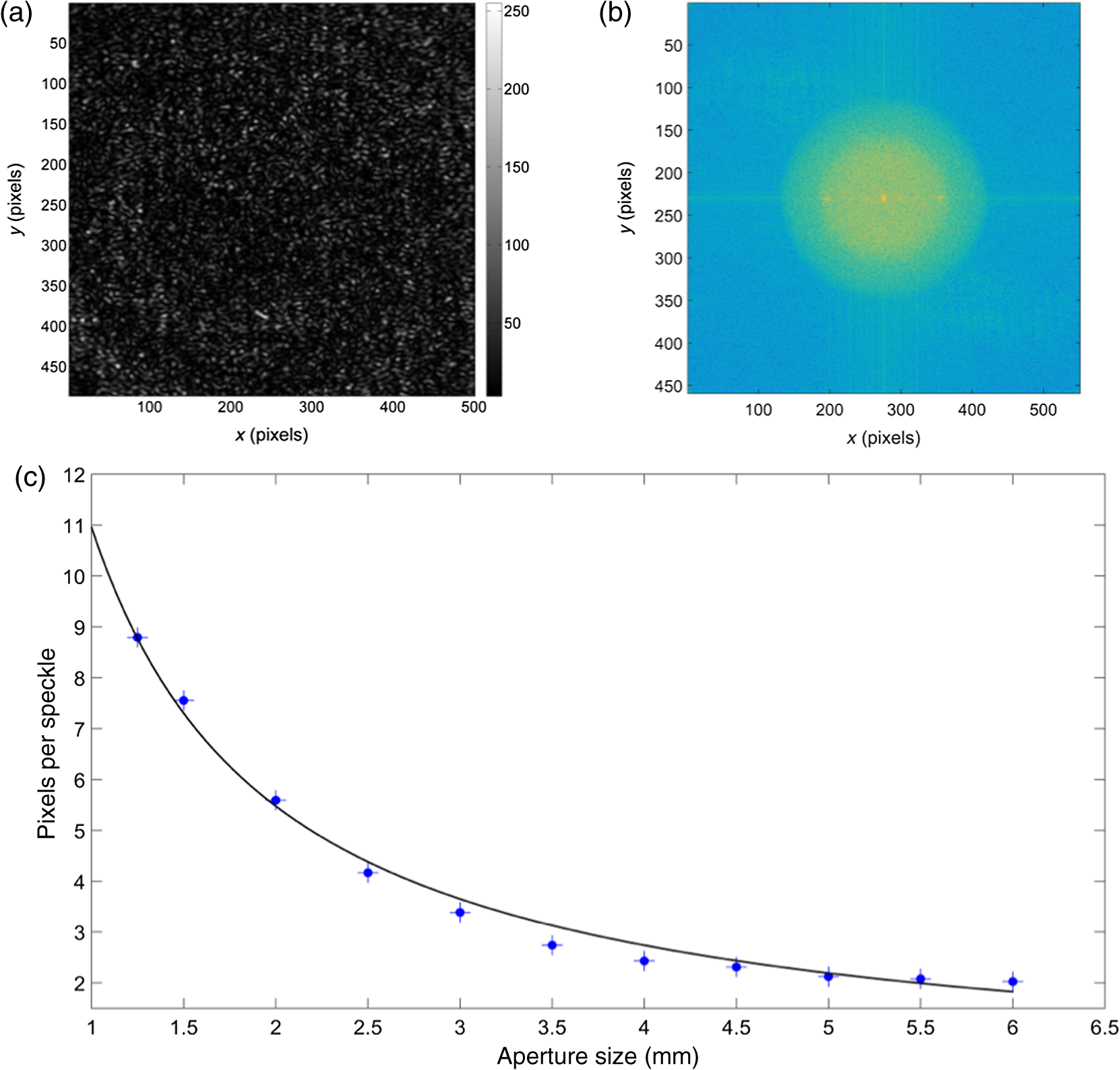

To generate an LSC image, multiple sequential frames of speckle patterns imaged by the CMOS array were summed to simulate speckle blurring, as seen when dynamic speckle is imaged with a finite exposure time. The blurred speckle results in reduced contrast seen in temporal averaging. Contrast, $K$, was defined as

Fig. 6

Simulated LSC image. The center region represents the “flow” region $({\tau }_{\mathrm{c}2})$. The contrast ratio between the static $({\tau }_{\mathrm{c}1})$ and dynamic region was 4.108 dB. In this figure, the contrast range was set between [0, 1.5]. The nearly concentric rings arose from reflections in the optical system.

In LSCI, the link between speckle contrast and flow can only be made if the flow distribution is known. However, the actual flow distribution of biological fluid is often unknown. Early work has assumed the flow of blood to exhibit either purely unordered (Lorentzian) or ordered (Gaussian) flow.^2,15,16 Theoretically, a Lorentzian velocity distribution is only appropriate for Brownian motion (purely random flow). Conversely, a Gaussian velocity distribution is technically only appropriate for purely ordered flow. In practical situations, it is likely that the true flow model is a mixture between the Lorentzian and Gaussian line shapes. In laser engineering terms, the convolution between these two line shapes is a Voigt profile, frequently referred to as a rigid-body model.³ Because assumptions are made to describe the fluid velocity distribution, the unambiguous quantification of flow velocity from contrast values is not yet possible. To model the fluid velocity distribution with this system, in addition to controlling the temporal decorrelation rate of the speckle images, we produce speckle sequences that decorrelate following a user defined function. We demonstrate this by producing speckle sequences that result in calculated contrast values that follow both Gaussian and Lorentzian distributions.¹ However, it should be noted that any desired function can be used to mimic whatever flow model is desired. The experimental contrast values were compared to the theoretical values as a function of the ratio of the speckle decorrelation time, ${\tau }_{\mathrm{c}}$, and the integration time, $T$. Here, the speckle decorrelation time, ${\tau }_{\mathrm{c}}$, was predetermined by the realization number of the generated phase screens, and the integration time, $T$, was determined by the number of summed frames. The results are shown in Fig. 7 which displays a comparison of theoretical and experimental results. For the experiments with varied intensity, 30 phase screens assuming a Gaussian decorrelation pattern were summed to ensure the LSC images were sampled and summed to appropriately mimic contrast values seen when imaging experimental dynamic speckle with a finite exposure time.

Fig. 7

SLM simulated contrast versus ${\tau }_{\mathrm{c}}/T$ for both a Gaussian and Lorentzian velocity distribution. The SLM setup was able to faithfully reproduce the expected results for both flow models.

To adjust the intensity of the interference pattern, an ND filter wheel covering two-orders of magnitude was placed in front of the 2.5 mW stabilized HeNe laser used in these experiments. A photodetector was placed in the imaging plane to calibrate the intensity of the light at the CMOS array for each filter value prior to image acquisition. The intensity calibration curve can be seen in Fig. 8. This calibration curve was used to relate the speckle contrast to a relative reduction of laser power density at the imaging plane. This approach serves as an attempt to generalize the results so that they may be applied to an array of LSCI applications where the scattering and absorption of light by tissue may result in backscattered light with varied intensities.

Fig. 8

Relation between ND filter and average intensity at CMOS array. The intensity was reduced logarithmically from the full intensity of $.0605\mathrm{mW}/{\mathrm{cm}}^2$.

To address the effects of over- and underexposing speckle during image acquisition, the exact same phase screens were loaded to the SLM and the resulting speckle patterns were imaged in the same sequence at each intensity value. The statistical behavior of a single “frozen” speckle pattern was assessed and then the contrast from the incoherent sum of 30 images was calculated. This summation of 30 images mimics a finite exposure time as would be used in an actual LSCI application.

Herein, we describe the effects of light intensity on sensitivity to changes in spatial decorrelation between “flow” and “static” regions. The ratio between the contrasts in the two regions is calculated in dB as

$K_{\text{static}}$ was calculated in a $200\times 100\text{pixel}$ area in the ${\tau }_{\mathrm{c}1}$ region, while $K_{\text{flow}}$ was calculated from a $200\times 100\text{pixel}$ area in the faster decorrelating, ${\tau }_{\mathrm{c}2}$ region.

3.

Results

An example of the same imaged “frozen” speckle pattern sampled at varying intensities can be seen in Fig. 9. The global spatial contrast of this speckle pattern, as calculated by Eq. (3), is shown across the full range of intensities investigated in Fig. 10(a), with the global intensity mean and spatial standard deviations used to calculate contrast plotted in Fig. 10(b). In the frozen speckle images where the mean intensity is approximately equal to the standard deviation (in the intensity range from 6.05 to $605\mu \mathrm{W}/{\mathrm{cm}}^2$, 10% to 1% of full intensity), the resulting contrast is close to the theoretical value of unity. The global contrast was closest to unity when the mean intensity value fell between grayscale values of 10 to 73 (recall that an 8-bit CMOS chip was used in these experiments). In practice, the contrast is rarely equal to the exact theoretical value of 1.0 due to mechanical vibrations, dark current noise in the system, and the fact that calculated global contrast values display an intrinsic log-normal distribution.¹⁷

Fig. 9

“Frozen” speckle patterns at (a) 100%, (b) 30%, (c) 8.75%, and (d) 3.4% of full intensity ($0.0605\mathrm{mW}/{\mathrm{cm}}^2$).

Fig. 10

(a) Contrast in a single speckle frame. In the case where a large number of speckles are used to calculate $K$ the theoretical limit of $K=1$ can be assumed as the “ideal.”¹¹ (b) The global mean intensity (black dots) and standard deviation (red stars) used to calculate contrast of a single speckle pattern.

The effects of incident intensity on the sampled first-order statistics of the individual speckle patterns were also investigated. Note that the random phase screens used to generate the speckle patterns had a phase modulation of $[0,2\pi ]$. Thus, since a single polarization state was observed, the speckle patterns produced from these phase screens should exhibit a negative exponential intensity PDF. The first-order statistics (PDFs) seen in the camera quantization of the speckle at the intensity extremes displayed deviation from the negative exponential in both the calculated PDF and in the camera intensity histogram, as seen in Fig. 11. The histograms show that high incident intensity results in pixel saturation while low intensities cover a smaller range of gray values. The highest contrast values were seen in the cases where both the calculated PDF and quantized intensities (histogram data) follow the theoretical negative exponential.

Fig. 11

PDF of speckle patterns at (a) 100%, (b) 30%, (c) 8.75%, (d) 1.1%, (e) 35%, and (f) 12% of full intensity, plotted on a log scale. Camera histogram of speckle patterns at (g) 100%, (h) 30%, (i) 8.75%, (j) 1.1%, (k) 35%, and (l) 12% of full intensity.

The resulting spatial contrast analysis, following the summation of the 30-image sequences at varied intensities, is shown in Fig. 12. The 200-pixel band in the center of the image displayed rapid blurring of the speckles, thus reducing contrast, as expected due to the smaller ${\tau }_{\mathrm{c}2}$. In this set of images, it is clear that there is an intensity range that results in optimal discrimination between the rapidly and slowly decorrelating regions. To quantitatively assess this, the contrast values of both the simulated “static” and “flow” regions were plotted in Fig. 13. The intensity values that resulted in a near theoretically ideal PDF in the “frozen” speckle patterns (1% to 10%) showed the highest contrast ratio between “static” and “flow” regions when the respective speckle patterns were summed. Within this range of intensities, the “frozen” speckle pattern exhibits a global contrast near unity. Outside of this range, the contrast values in the “dynamic” speckle vary and sensitivity to speckle motion become reduced.

Fig. 12

Spatial analysis of speckle patterns at intensities of (a) 100%, (b) 30%, (c) 8.75%, (d) 3.4%, (e) 1.1%, and (f) 35%. The ring in the upper right corner of the images comes from statistically negligible noise in the optical system.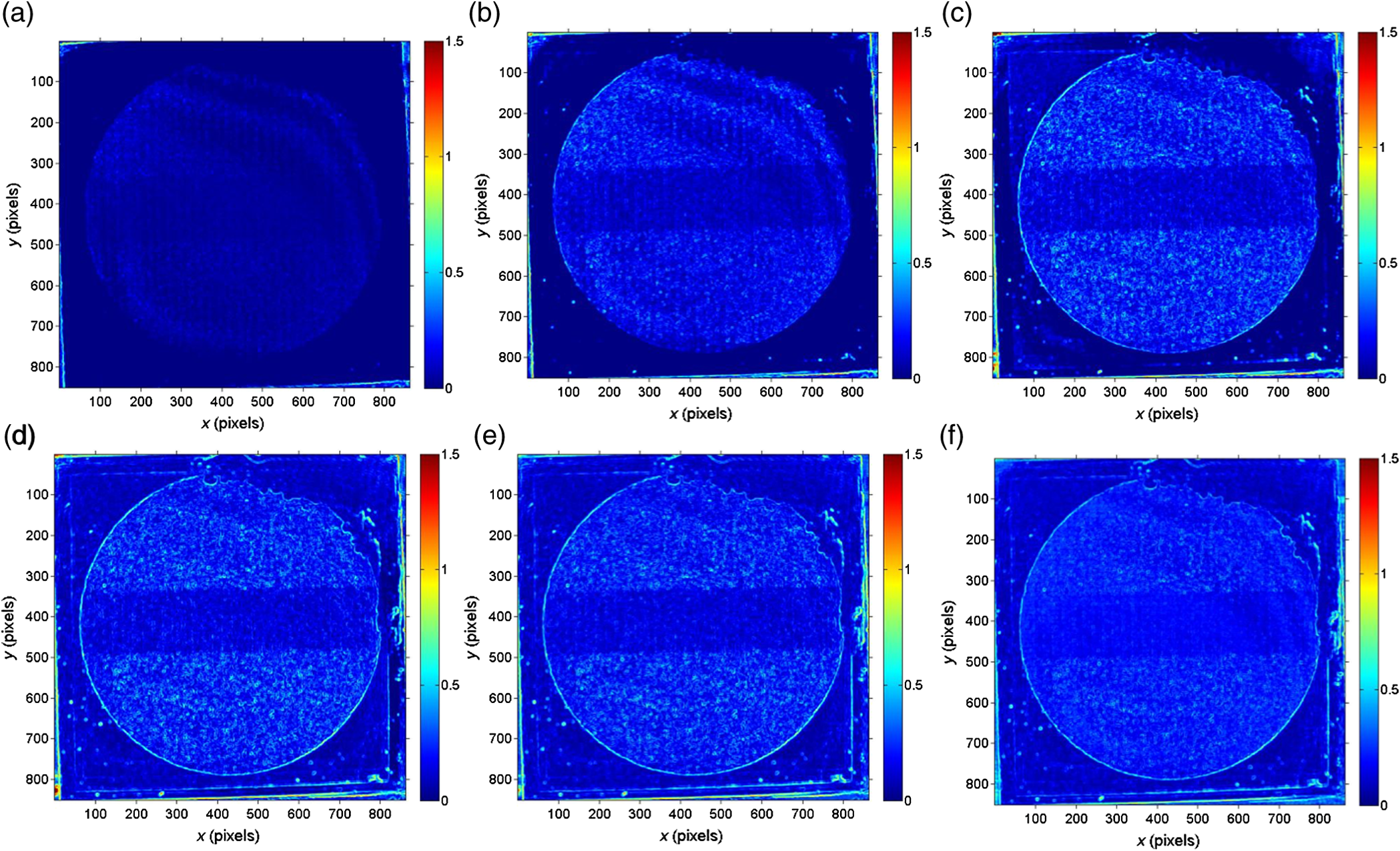

Fig. 13

(a) Contrast of speckle regions in spatial averaged LSCI. Red stars indicate the “flow” region of faster decorrelating speckle, with the black dots indicative of the “tissue” region with slower decorrelating speckle. (b) Contrast ratio of the “flow” region and the “static” region. Optimum sensitivity to temporal changes follows the trends in Fig. 10.

By assessing the width of the PSD of the individual speckle patterns, the frequency content of the images can be assessed. For an appropriately (spatially) sampled speckle image, with no saturation or significant underexposure, the frequency content is a means of estimating the minimum speckle size in the speckle image (i.e., second-order statistics). Since the minimum speckle size was set during the course of the experiments by the diameter of the aperture in the imaging arm, we were able to use this a priori information to investigate the effects of image saturation on the frequency content of the speckle images. An intensity trace was plotted across the PSD and the full width half max (FWHM) was estimated to get the width of the PSD, and thereby address the effects of saturation on the frequency content of the speckle images. The “apparent” imaged speckle size, artificially created by the loss of high frequency content, was calculated by taking the FWHM of the PSD and dividing the result by 2 (because DC is located in the center of the display) so the values used align with the theoretical calculation of speckle size seen in Eq. (1). The experimentally determined “apparent” speckle size was then normalized relative to the camera pixel size and shown in Fig. 14. A loss of high frequency data was seen in speckle patterns imaged with greater than 10% of full intensity. This result indicates that there may be pixel saturation at higher intensities.¹⁸

Fig. 14

(a) PSD of frozen speckle pattern imaged at 8.75% of full intensity, (b) intensity profile through the center of (a). (c) Frequency information was used to calculate “apparent” speckle size at each incident intensity. The “apparent” increase in speckle size was actually a loss of high frequency content in the image due to saturation.

In many applications of LSCI, raw speckle images are subject to histogram equalization so as to fill the full dynamic range prior to processing.^19,20,21 This scaling effect often adjusts the mean contrast in the single speckle pattern, and it is thought to improve an underexposed image. To assess whether the simple histogram equalization results in improved contrast, the gray values of each imaged speckle pattern summed in the spatial contrast analysis of “dynamic” speckle were scaled to fill the full dynamic range of the camera. Another approach would be to employ a higher bit-camera and bin multiple intensity values so as to reduce the number of gray levels. However, the goal of this simple analysis is to briefly display that although single “frozen” speckle look better post equalization, the actual image quality is not improved. For this investigation, the exact same speckle patterns were adjusted to ensure the only altered variable was the scaling function. The spatial contrast analysis on the scaled images resulted in an almost identical range of optimal values as a function of intensity. A comparison of scaled and unscaled contrast values can be seen in Fig. 15. Figure 15 also shows an example of the scaled histogram data from a speckle pattern at a very low intensity (0.03% of full intensity). The resulting measured contrast values following the histogram equalization were nearly identical to the contrast values of the unscaled speckle patterns in the resulting spatial contrast analysis. The results indicate that simple histogram equalization does not significantly improve speckle statistics and sensitivity to flow at low intensities.

Fig. 15

Raw speckle data imaged at 0.35% intensity: (a) histogram scaled, (b) contrast values shown with all images scaled to fill the full dynamic range of the 8-bit camera. The optimum imaging window of incident intensity showed little to no difference in the spatial analysis between the original (red stars) and scaled (blue triangles) images. (c) Contrast ratio of the “flow” region and the “static” region for both scaled (blue triangle) and unscaled (red star) speckle.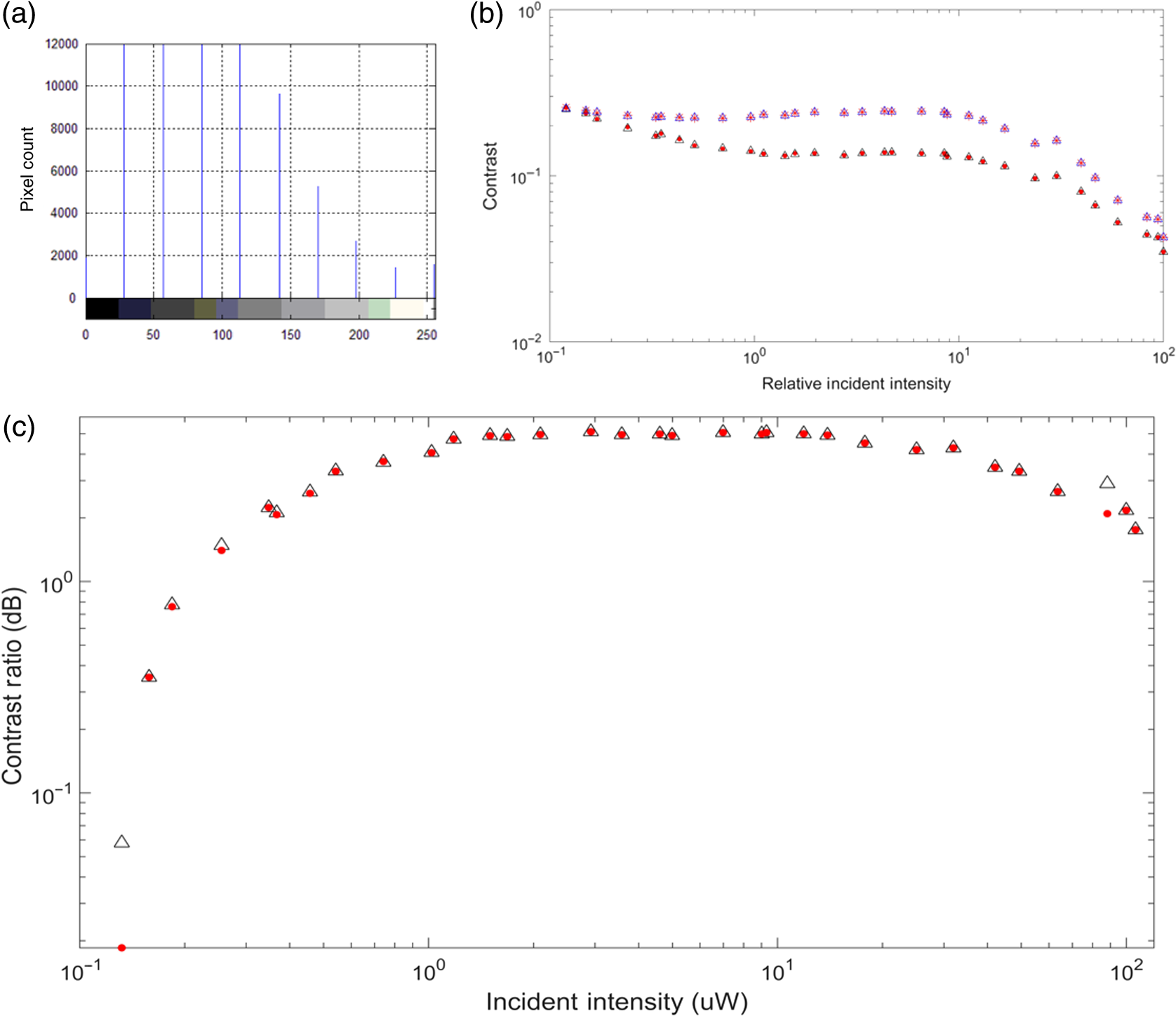

4.

Conclusions

The results of our experiments indicate that there is a range of incident intensities that approach the theoretically ideal PDF for fully developed speckle. This in turn corresponds to a global contrast approaching unity. When the single speckle patterns displayed characteristics near the theoretically ideal values, the resulting spatial contrast analysis from a summation of speckle patterns displayed a high sensitivity to motion. The results indicate the importance of assessing the quantized signal and resulting intensity PDF of the speckle patterns during image acquisition in LSCI. The optimum sensitivity of the LSC image is seen when the speckle frames have appropriate intensity distribution to display the first-order statistics of fully developed speckle.

It is clear that at high intensities, high frequency information is lost due to camera saturation, resulting in a decrease in contrast. In cases of high incident intensity, it has been proposed that intensity peaks are clipped in the quantization process of the camera.¹⁸ When the average intensity of the raw speckle image is less than half the maximum intensity value of the sensor, clipping of the intensity peaks is assumed to have a reduced effect. For an 8-bit camera with $2^8=256$ different gray values, Alexander et al.¹⁸ proposed that the maximum average intensity value should be 128 to avoid clipping of high frequency data. That is, the maximum average gray level should be no more than 128 in order to avoid saturation and the loss of the ability to resolve individual speckles. Our results support this claim. At higher intensities, the imaged speckle displayed decrease in high frequency content due to pixel saturation. When the average intensity gray value was above 125 ($>16\%$ of the full intensity), we also saw a reduction in statistical variance that resulted in contrast values diverging from the theoretical maximum. It is also worth noting that detecting the number of saturated pixels in the image, prior to spatial contrast analysis could serve as a method to determine if the camera is oversaturated. Others have indicated that increased intensity improves detectability of changes to flow;²² however, our results indicate that there is a window of laser power densities that result in optimum sensitivity. In practice, the upper range of incident light intensity is limited by the laser power density at which a coherent light source will backscatter without inducing functional changes in the tissue due to global absorption. In other words, the laser power density where functional changes occur in the tissue is the limiting factor in determining a maximum incident intensity. At this maximum incident intensity, a combination of reducing the imaging aperture diameter and shortening the camera integration time can be used to prevent saturation.

Simply scaling to fill the full dynamic range using an 8-bit camera improved the mean intensity when the images were underexposed, but did not correct for the loss of data due to the digital quantization process. Even though this process improved the mean intensity value, the standard deviation changed at relatively the same rate, resulting in little to no improvement in calculated contrast. If the gray values of underexposed images are quantized by a lower bit system, small variances in the shades of gray may be binned to the same gray value, resulting in a loss of information. Simple histogram equalization does not improve contrast data in a situation where sampling results in information loss. However, there may be reason to further explore methods of preprocessing speckle data so as to improve the statistics of poorly sampled data. There have been proposed methods to solve the issue of uneven illumination that may be applied to improve the contrast of underexposed images used in LSCI.^23,24,25 It can also be reasoned that increased camera bit-depth may result in fully developed speckle characteristics and optimum sensitivity across a wider range of incident intensity values.²³ In practice, however, adjusting the incident intensity and camera settings may be sufficient to ensure optimal speckle statistics are satisfied when sampling speckle data for LSCI.

We have shown the ability of our system to faithfully reproduce the speckle images used in LSC imaging and its promise as a research tool. Because our electro-optical system allows for fast experimentation and reproduction, this system provides a convenient and quantifiable platform to address many of the real-world complications that hinder the on-going development of LSCI, such as incident intensity in experimental settings. It is hoped that through approaches similar to that employed herein, the fine details of LSCI can be explored in more detail and further development of the imaging modality as a reliable and inexpensive research and diagnostic tool can proceed.