
|
|
1.IntroductionQuantitative and label-free measurement of microvascular flow velocity is significant for diagnostic and therapeutic purposes because the flow velocity is an indicator of circulatory system diseases, such as arterial hypertension, ischemia inflammation, and diabetes.1–3 The capability to obtain high spatial resolution images and accurate velocity values has made optical imaging suitable for such a kind of measurement. The related methods include double-slit photometry,4 laser Doppler velocimetry,5 photoacoustic correlation spectroscopy,6 Doppler optical coherence tomography,7–9 autocorrelation optical coherence tomography,10 and dynamic light scattering.11,12 All these methods work in a point-to-point scanning mode. Full-field optical imaging has the advantage in getting the dynamic information of RBCs in a frame simultaneously. A typical example is laser speckle contrast imaging, with which one realizes blood flow velocity mapping.13 On the other hand, autocorrelation analysis in microscopy systems can be used for tracking individual RBC motions in transparent media and extracting their velocities.14,15 In this paper, we propose an improved full-field autocorrelation imaging method, i.e., spatiotemporal demodulation autocorrelation (SDA), to quantify the velocities of RBCs in capillaries. Particularly, an RBC signal is first demodulated from the background signal by temporal demodulation. To improve the contrast ratio of RBC to background, the RBC signal is further processed with the Butterworth spatial filter. The process above is the so-called spatiotemporal demodulation (SD). Then, based on the extracted RBC signal, lag time and RBC length are obtained by autocorrelation analysis and image segmentation, respectively. Finally, RBC velocity is derived according to the ratio of RBC length to lag time. We would like to make three remarks. The first is that, different from the conventional velocity imaging methods based on autocorrelation analysis, which ignore the RBC length variation related to the RBC location, SDA takes this variation into consideration; thus, the RBC velocity obtained is more accurate. The second is that SD significantly increases the image signal-to-noise ratio (SNR) by weakening the negative influence of background and noise so that autocorrelation analysis can be used for the turbid tissue. The third is that our full-field velocity imaging method with a microscopy system can be used to observe all the RBC shapes, orientations, and velocities at different locations of capillaries simultaneously. 2.Material and Theory2.1.System Setup and Animal PreparationIn the present investigation, an optical microscope system (MF-UA1010C) was employed as the imaging apparatus. A matrix CMOS camera (Aca2040-180kmNIR, Basler) with exposure time of and sampling rate of 370 fps was used to acquire 512 images. The pixel size of the camera was . The whole imaging apparatus was fixed on a vibration-free optical platform. 2.2.Spatiotemporal Demodulation AutocorrelationIn the following, we would like to show how we calculate RBC velocity by SDA. When RBCs pass through the image field of each pixel one by one with, sometimes, large separation, they continuously scatter the probe beam. This results in the formation of light pulses. The acquired signal intensity can be approximated by where is the scattering intensity from the background, is the noise, and describes the RBC scattering light needed for calculating RBC velocity. In theory, relates to the amplitude, which can be considered a constant; is a unit rectangle function with width and beginning time when the ’th RBC passes through the concerned location;10 and is the number of RBCs passing through the location of interest. For turbid tissue, RBC signal is buried by the background and noise ; thus, it is difficult to measure RBC length and velocity directly with raw data. In order to extract the RBC signal, we perform a fast Fourier transform (FFT) on the acquired raw signal and obtain the frequency-domain RBC signal . where means the band-pass filter with and being the cut-off frequencies. In the frequency domain, the background signal mainly locates at zero frequency, and the RBC signal frequency determined by the RBC velocity is in the range of to . In theory, , where is the sampling rate of the camera and is the number of acquisition frames. , where is the maximum number of RBCs passing through a pixel during the acquisition time . Then, by applying an inverse FFT to Eq. (2), we obtain the time-domain RBC signal. can be considered approximately in Eq. (1). Furthermore, we introduce the Butterworth spatial filter to increase the contrast ratio of RBCs and the background. After all the operations above, the RBC signal is suitable for the velocity calculation.RBC velocity can be derived by the formula , where is the RBC length calculated by image segmentation, is the lag time for RBCs passing through a pixel and can be obtained by autocorrelation analysis, and its reciprocal, , is equal to the slope of the autocorrelation curve from the origin to the first zero of the ordinate.6,10 The autocorrelation curve is obtained by performing autocorrelation analysis on the data processed by SD. How to calculate RBC length is described in Sec. 3.2. 3.Results and Discussion3.1.Method ValidationThe following experiment is designed to verify that the SD operation has less negative influence on the accuracy of the lag time calculation with the autocorrelation algorithm. The experiment was on a resolution test target (DOFH 5-15-50-80). Here, the target was approximately perpendicular to the probe beam and was controlled by a linearly motorized stage to move at a speed from 0.1 to with an interval of . Figure 1(a) presents the SD image of the target. After being modulated by the moving stripes on the target, the acquired signals become a series of pulses, simulating the scattering lights from the RBCs passing through a capillary. The lag time obtained by the conventional autocorrelation analysis can be taken as a reference. Figure 1(b) shows the relationship between the velocity and lag time obtained by conventional autocorrelation analysis (solid line) and SDA (dotted line), respectively. Evidently, the result obtained by SDA is in good agreement with that only by autocorrelation analysis. Therefore, the SD operation is feasible. Fig. 1(a) SD image of resolution test target; (b) velocity–lag time curves obtained by conventional autocorrelation analysis (solid line) and SDA (dotted line). 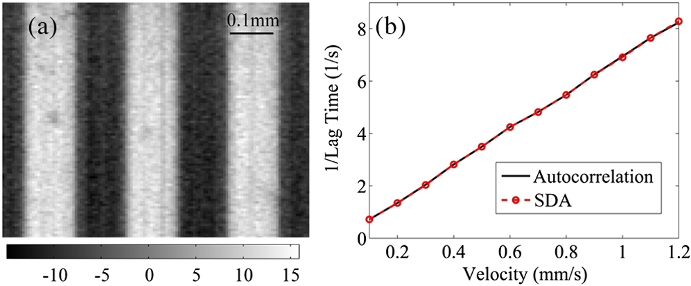 After the above verification, we demonstrate by the following experiment on an in vivo mouse ear that the image SNR and the accuracy of autocorrelation algorithm increase after the SD operation. The 1-month male mouse weighing 16 g was anesthetized with 10% chloral hydrate (0.08 mL) and its ear was depilated with a hair remover lotion. The animal procedures were performed under a protocol approved by the Institutional Animal Care and Use Committee at Beijing Normal University. Figure 2(a) shows the raw blood flow image. Because the RBC signal is buried by the background signal, the locations of the RBCs cannot be identified easily. Figure 2(b) presents the image obtained by temporal demodulation, where RBCs appear, and in Fig. 2(c), the image is processed further by the Butterworth spatial filter, where the contrast ratio of background to RBCs is higher. The SD performance can be illustrated more clearly by comparing the raw movie (see Video 1) with the SD movie (see Video 2). In order to analyze the image SNR, we present in Figs. 2(d)–2(f) the temporal signals at A as indicated correspondingly in Figs. 2(a)–2(c). In these figures, the inverse peaks appear at the moments when RBCs pass through A. Image SNR is defined as where means the absolute value, stands for the average value of the RBC signal, and is the average value of the background signal. In our case, and can be decided in the following way. If we take [see the horizontal line in Fig. 2(d)] as the average value of the temporal signal, the RBC signal has a value smaller than and a background signal higher than . According to Eq. (4), the SNR of the raw image [Fig. 2(a)] is 0.64 dB, while that of the SD image is 10 dB, increasing about 16 times. The corresponding autocorrelation curves are shown in Figs. 2(g)–2(i). Apparently, based on the autocorrelation curve in Fig. 2(i), the lag time can be calculated more accurately.Fig. 2(a) Raw, (b) temporal demodulation, and (c) SD images of capillaries; (d) through (f) temporal signals at A in (a) through (c); (g) through (i) autocorrelation curves of temporal signals in (d) through (f). , indicated by the horizontal line in (d), is the average value of temporal signal. and are RBC signal and background signal, respectively. The details of RBC movement in capillaries can be seen in the raw movie (Video 1, MOV, 9231 KB) [URL: http://dx.doi.org/10.1117/1.JBO.21.3.036007.1]. and SD movie (Video 2, MOV, 9054 KB) [URL: http://dx.doi.org/10.1117/1.JBO.21.3.036007.2].  3.2.Red Blood Cell Length CalculationRBC length is another factor crucial to the RBC velocity calculation. Figure 3 demonstrates how the RBC length at different locations in capillaries is extracted. First, we identify capillaries in which RBCs flow. To this end, we use intensity fluctuation modulation (IFM), which was first proposed in laser speckle angiography.16,17 The main idea of IFM is that the information of blood flow can be obtained by separating the dynamic signal, which is related to the moving RBCs in the blood flow, from the stationary signal, which is related to the background tissue. In the present case, the dynamic signal is just and the stationary signal is in Eq. (1). Figure 3(a) is an IFM image where the capillaries are resolved, and Fig. 3(b) is the image obtained after performing image segmentation on the IFM image. Then, combining the segmented IFM image and the SD image [see Fig. 2(c)], we can segment and track the RBCs almost free from the background disturbance. How to trace the RBC motion is shown in the supplementary movie (see Video 3), from which the variations of the RBC shape, orientation, and size can be seen clearly. In order to facilitate observation, we present one of the respective frames of the movie, a segmented RBC image [Fig. 3(c)], to display the RBC distribution in the capillaries. One can decide the length of an RBC simply by measuring its size along its moving direction. Finally, RBC length for a pixel is given by the value averaged over all the lengths of the RBCs passing through this pixel. Fig. 3(a) IFM image, (b) segmented IFM image, and (c) segmented RBC image where an arrow indicates RBC length . The segmented RBCs can be traced in the movie (Video 3, MOV, 2460 KB) [URL: http://dx.doi.org/10.1117/1.JBO.21.3.036007.3].. (d) Segmented SD-RBC image where RBCs are outlined. The rectangle indicates out-of-focus region. The dynamic process of the RBCs marked by their outlines can also be observed in the movie (Video 4, MOV, 9028 KB) [URL: http://dx.doi.org/10.1117/1.JBO.21.3.036007.4]. 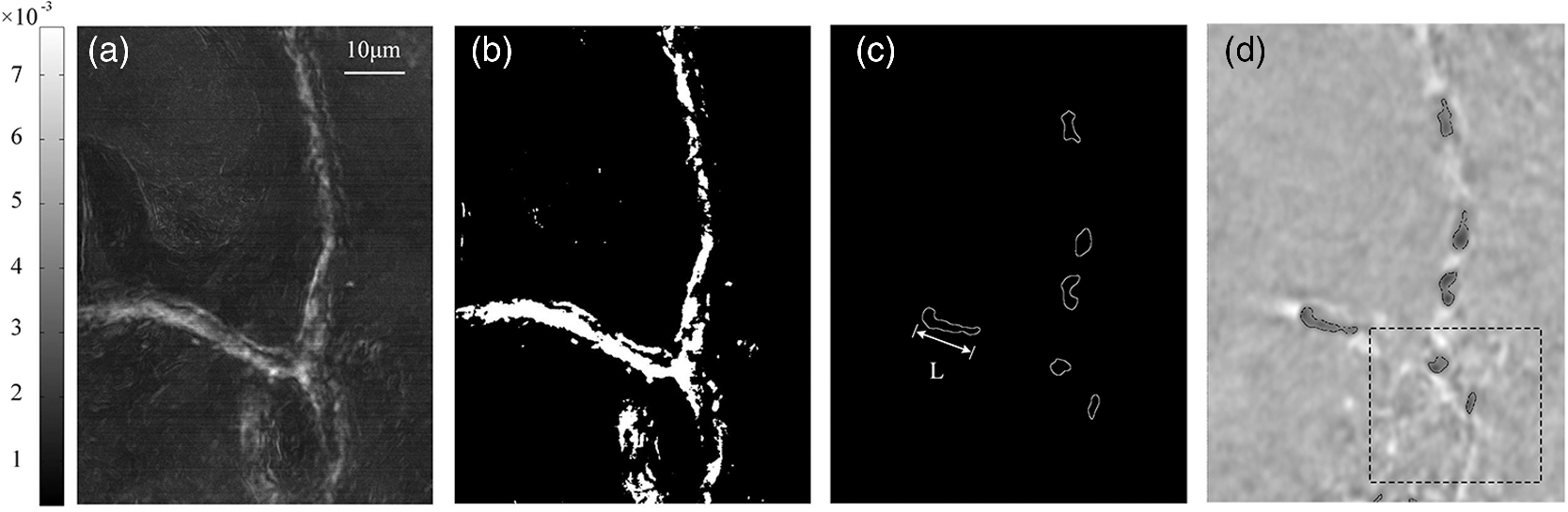 In a real case, the length of an RBC, the one indicated by the arrow in Fig. 3(c), for example, is determined by the outline of this RBC. Figure 3(d) presents the segmented SD-RBC obtained by superposing the segmented RBC image on the SD image. In this figure, each outline represents an RBC. More detailed information about all RBCs can be obtained in the movie (see Video 4), which fully demonstrates the effectiveness of our method for tracing RBCs and obtaining their lengths. We note here that our imaging depth is limited due to our microscopy system with a short focus. Thus, for the capillary that locates in the defocused area, our method will fail. The area indicated by the dashline rectangle in Fig. 3(d) is just in this case. The problem could be solved by using depth scanning. On the other hand, because of the working mode of white light, short focus, and vertical incidence in our experiment, the influence of the Doppler angle on the measurement can be ignored, and the achieved RBC velocity can be considered approximately the absolute velocity. 3.3.Velocity ImagingFigure 4 presents the segmented IFM images marked with [Fig. 4(a)], RBC length [Fig. 4(b)], and RBC velocity [Fig. 4(c)]. If the difference between any two RBC lengths is neglected, Fig. 4(a) can be taken as the RBC velocity distribution. Of course, this is inaccurate. Statistically, Fig. 4(b) describes the length variation of an RBC at different locations in a capillary. Similarly, Fig. 4(c) describes the velocity variation of an RBC at different locations. The velocities of RBCs in different capillaries, those indicated by red and blue arrows, for example, are apparently different. These phenomena can be clearly observed in Videos 2 through 4 and are in accord with our observation made in the real situation. The fact above tells us again that it is accurate to calculate RBC velocity based on the assumption that both RBC length and lag time are variables. 4.ConclusionWe propose a full-field imaging method called SDA for mapping the velocities of RBCs in capillaries with a white-light microscopy system. Here, SD is adopted to separate the RBC signal from the background signal and noise, with which it becomes possible to extract the RBC length by image segmentation, the lag time by autocorrelation analysis, and, finally, the velocities of RBCs. The performance of our method is verified by an experiment on an in vivo mouse ear. Our method may have potential applications in the quantitative analysis of cerebral blood flow dynamics and the study of different patterns of brain capillary network flow between a healthy brain and a pathological brain, for instance, the brain affected by Alzheimers disease. It might also be used in the study of cellular metabolism and embryo viability. AcknowledgmentsThis work is subsidized by the National Natural Science Foundation of China, Project Nos. 11174040, 61008063, and 61275214. ReferencesG. Mchedlishvili and N. Maeda,
“Blood flow structure related to red cell flow: a determinant of blood fluidity in narrow microvessels,”
Jpn. J. Physiol., 51 19
–30
(2001). http://dx.doi.org/10.2170/jjphysiol.51.19 Google Scholar
K. Cruickshank et al.,
“Aortic pulse-wave velocity and its relationship to mortality in diabetes and glucose intolerance: an integrated index of vascular function,”
Circulation, 106 2085
–2090
(2002). http://dx.doi.org/10.1161/01.CIR.0000033824.02722.F7 CIRCAZ 0009-7322 Google Scholar
K. Fassbendera et al.,
“Inflammatory cytokines in subarachnoid haemorrhage: association with abnormal blood flow velocities in basal cerebral arteries,”
J. Neurol. Neurosurg. Psychiatry, 70 534
–537
(2001). http://dx.doi.org/10.1136/jnnp.70.4.534 Google Scholar
H. Wayland and P. C. Johnson,
“Erythrocyte velocity measurement in microvessels by a two-slit photometric method,”
J. Appl. Physiol., 22 333
–337
(1967). Google Scholar
M. D. Stern,
“Laser Doppler velocimetry in blood and multiply scattering fluids: theory,”
Appl. Opt., 24 1968
–1986
(1985). http://dx.doi.org/10.1364/AO.24.001968 APOPAI 0003-6935 Google Scholar
S. L. Chen et al.,
“Photoacoustic correlation spectroscopy and its application to low-speed flow measurement,”
Opt. Lett., 35 1200
–1202
(2010). http://dx.doi.org/10.1364/OL.35.001200 OPLEDP 0146-9592 Google Scholar
S. G. Proskurin, Y. H. He and R. K. Wang,
“Determination of flow velocity vector based on Doppler shift and spectrum broadening with optical coherence tomography,”
Opt. Lett., 28 1227
–1229
(2003). http://dx.doi.org/10.1364/OL.28.001227 OPLEDP 0146-9592 Google Scholar
R. K. Wang and Z. Ma,
“Real-time flow imaging by removing texture pattern artifacts in spectral-domain optical Doppler tomography,”
Opt. Lett., 31 3001
–3003
(2006). http://dx.doi.org/10.1364/OL.31.003001 OPLEDP 0146-9592 Google Scholar
R. M. Werkmeister et al.,
“Bidirectional Doppler Fourier-domain optical coherence tomography for measurement of absolute flow velocities in human retinal vessels,”
Opt. Lett., 33 2967
–2969
(2008). http://dx.doi.org/10.1364/OL.33.002967 OPLEDP 0146-9592 Google Scholar
Y. Wang and R. K. Wang,
“Autocorrelation optical coherence tomography for mapping transverse particle-flow velocity,”
Opt. Lett., 35 3538
–3540
(2010). http://dx.doi.org/10.1364/OL.35.003538 OPLEDP 0146-9592 Google Scholar
C. Joo et al.,
“Diffusive and directional intracellular dynamics measured by field-based dynamic light scattering,”
Opt. Express, 18 2858
–2871
(2010). http://dx.doi.org/10.1364/OE.18.002858 OPEXFF 1094-4087 Google Scholar
A. B. Leung, K. I. Suh and R. R. Ansari,
“Particle-size and velocity measurements in flowing conditions using dynamic light scattering,”
Appl. Opt., 45 2186
–2190
(2006). http://dx.doi.org/10.1364/AO.45.002186 APOPAI 0003-6935 Google Scholar
S. Dufour et al.,
“Evaluation of laser speckle contrast imaging as an intrinsic method to monitor blood brain barrier integrity,”
Biomed. Opt. Express, 4 1856
–1875
(2013). http://dx.doi.org/10.1364/BOE.4.001856 BOEICL 2156-7085 Google Scholar
A. G. Koutsiaris, D. S. Mathioulakis and S. Tsangaris,
“Microscope PIV for velocity-field measurement of particle suspensions flowing inside glass capillaries,”
Meas. Sci. Technol., 10 1037
(1999). http://dx.doi.org/10.1088/0957-0233/10/11/311 MSTCEP 0957-0233 Google Scholar
Y. Sugii, S. Nishio and K. Okamoto,
“In vivo PIV measurement of red blood cell velocity field in microvessels considering mesentery motion,”
Physiol. Meas., 23 403
(2002). http://dx.doi.org/10.1088/0967-3334/23/2/315 PMEAE3 0967-3334 Google Scholar
Y. G. Zeng et al.,
“Laser speckle imaging based on intensity fluctuation modulation,”
Opt. Lett., 38 1313
–1315
(2013). http://dx.doi.org/10.1364/OL.38.001313 OPLEDP 0146-9592 Google Scholar
M. Y. Wang et al.,
“Full-field optical micro-angiography,”
Appl. Phys. Lett., 104 053704
(2014). http://dx.doi.org/10.1063/1.4864156 APPLAB 0003-6951 Google Scholar
Biography |


