Division of focal plane polarimeter-based 3 × 4 Mueller matrix microscope: a potential tool for quick diagnosis of human carcinoma tissues

Jintao Chang; Honghui He; Ye Wang; Yi Huang; Xianpeng Li; Chao He; Ran Liao; Nan Zeng; Shaoxiong Liu; Hui Ma

doi:10.1117/1.JBO.21.5.056002

9 May 2016 Division of focal plane polarimeter-based 3 × 4 Mueller matrix microscope: a potential tool for quick diagnosis of human carcinoma tissues

Jintao Chang, Honghui He, Ye Wang, Yi Huang, Xianpeng Li, Chao He, Ran Liao, Nan Zeng, Shaoxiong Liu, Hui Ma

Author Affiliations +

Journal of Biomedical Optics, Vol. 21, Issue 5, 056002 (May 2016). https://doi.org/10.1117/1.JBO.21.5.056002

Abstract

A polarization microscope is a useful tool to reveal the optical anisotropic nature of a specimen and can provide abundant microstructural information about samples. We present a division of focal plane (DoFP) polarimeter-based polarization microscope capable of simultaneously measuring both the Stokes vector and the 3×4 Mueller matrix with an optimal polarization illumination scheme. The Mueller matrix images of unstained human carcinoma tissue slices show that the m₂₄ and m₃₄ elements can provide important information for pathological observations. The characteristic features of the m₂₄ and m₃₄ elements can be enhanced by polarization staining under illumination by a circularly polarized light. Hence, combined with a graphics processing unit acceleration algorithm, the DoFP polarization microscope is capable of real-time polarization imaging for potential quick clinical diagnoses of both standard and frozen slices of human carcinoma tissues.

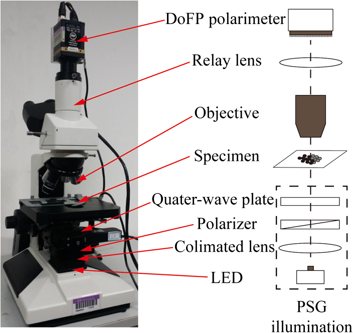
1. Introduction

Polarization imaging is becoming an emerging technique for studies in material,¹^,² astronomy,³ remote sensing,⁴^,⁵ and biomedicine.⁶^–⁹ When observing the biomedical and material specimens, polarization microscope is a useful tool to reveal their optical anisotropic nature and can provide abundant microstructural information about samples. The traditional polarization microscope adopts a polarizer to provide linear polarized illumination, and an analyzer is inserted for observation in cross- or parallel-polarized light mode, which is simple to implement but difficult for quantitative analysis.¹⁰ Oldenbourg et al.¹¹ modified the traditional polarization microscope by adopting the liquid crystal retarders. The modified microscopy greatly improves the analytic power, providing quantitative birefringence distributions of thin specimens, such as the mitotic spindle isolated from the fertilized sea urchin egg.¹¹ Recently, Arteaga et al.¹² proposed a Mueller matrix microscope based on two continuous rotating wave plates to completely extract the polarization property of a specimen. In this scheme, the intensity at each pixel is analyzed by digital demodulation of thousands of continuously captured frames.¹² The polarization microscopes based on liquid crystal retarders and rotating wave plates are division of time technologies, which are suitable for stationary samples. For the polarization measurements of dynamic processes, however, division of the focal plane (DoFP) polarimeters can be adopted. For a microgrid polarizer DoFP polarimeter, an array consisting of numerous differently orientated pixel-size micropolarizers is fixed on the imaging sensor.¹³^–¹⁵ Several recent studies have incorporated the DoFP polarimeter into a microscope for simultaneous Stokes vector imaging.¹³^,¹⁶ Liu et al.¹³ developed a complementary fluorescence-polarization microscope using a DoFP polarimeter to enable real-time video rate polarization imaging without any moving parts. Hsu et al.¹⁶ presented a polarization microscope using an infrared full-Stokes imaging polarimeter. The DoFP polarimeter has the same instrument size as the conventional image sensor and can capture the Stokes vector images in a single shot.

Recently, polarization imaging techniques have been used as potential tools for biomedical diagnosis, such as the detection of abnormal tissues in skin,¹⁷^,¹⁸ liver,¹⁹^,²⁰ esophagus,²¹ colon,²²^,²³ cervix,²⁴ bladder,²⁵ and so on.²⁶^–²⁸ Nowadays, the cancer incidence is growing fast worldwide, making pathological diagnoses time-consuming. Basically, during a diagnosis process, the pathologists need about half an hour to prepare the stained frozen slices of suspicious tissue samples from the patients. With careful observations using a transmission microscope, the pathologists need to provide quick assessments which are crucial for the surgeons. Compared to the diagnosis using the standard dewaxed slices cut from fixed tissues in paraffin specimens, the quick assessments always lead to a small portion of misdiagnose. In our experiments, we find that when using a DoFP polarimeter for polarization imaging of pathological tissue slices, the experimental results can provide additional useful information but will sometimes be confusing and misleading if the illumination state of polarization (SoP) and the sample are not well matched. For different illumination SoPs, there will be considerable differences in the specimen’s Stokes vector images. In this situation, measuring the sample’s Mueller matrix is conducive to our understanding of the sample’s comprehensive polarization property. Moreover, it is also found that when applied to the thin dewaxed slices of tissues, the intrinsic anisotropic fibrous structures of the cancerous tissues are more prominently highlighted in the Mueller matrix elements related to the circularly polarized light, or the elements in the fourth row and column. Hence, a DoFP polarimeter-based microscope capable of measuring the $3 \times 4$ Mueller matrix may provide useful information of human carcinoma tissue slices.

In this article, we propose an optimal 4-SoP illumination scheme for the $3 \times 4$ Mueller matrix measurement using a DoFP-based polarization microscope. The experimental results show that the polarization features of the unstained human carcinoma tissue slices are more prominently reflected in the Mueller matrix elements $m_{24}$ and $m_{34}$ . It is also indicated that the pathological microstructures are less visible in the polarization images under illumination by the linear polarization light, but can be enhanced by “polarization staining” under illumination by a circularly polarized light. As a nonstained technique, the DoFP-based polarization microscope can provide additional microstructural information of both standard and frozen pathological slices, which may be used as a potential tool for the quick diagnosis of human carcinoma tissues.

2. Methods and Materials

2.1.

Polarization Imaging Using the Division of Focal Plane Polarimeter

We use the DoFP polarimeter “PolarCam” (4D Technology Inc.) whose sensor size is $488 \times 648 pixels$ and whose video frame rate can reach to 110 fps.¹⁵ The diagram of the pixelated micropolarizer array is shown in Fig. 1(a). Four pixels with different polarization orientations comprise a super pixel, which are combined together to calculate the linear part of the Stokes vector

Eq. (1)

S = [\begin{matrix} S_{0} \\ S_{1} \\ S_{2} \end{matrix}] = [\begin{matrix} I_{0} + I_{90} \\ I_{0} - I_{90} \\ I_{45} - I_{135} \end{matrix}],

where

I_{0}

,

I_{45}

,

I_{90}

, and

I_{135}

are the intensities of the linear polarization components at four different degrees. Since for a DoFP polarimeter, the image sensor response, the extinction ratio, and the transmission axis of each pixel inherently have significant nonuniformities, calculating the Stokes vector simply using Eq. (1) would introduce errors.²⁹ For accurate Stokes vector measurement, the nonuniformities for all pixels should be calibrated. We introduce light with different known SoPs and measure the instrument responses to obtain the instrument matrix of the polarimeter.³⁰ Using the obtained instrument matrix, we can calculate the Stokes vector using the polarimetric data reduction method. For each super pixel as shown in Fig. 1(a), the polarimetric measurement can be expressed as

Eq. (2)

I = A \cdot S,

where

I

is the light intensity of the four pixels and

A

is a

4 \times 3

instrument matrix for a super pixel. Then

S

can be calculated by

S = pinv (A) \times I

, where pinv (

A

) represents the pseudoinverse of

A

. It has been shown that if the condition number (CN: the ratio of the largest singular value to the smallest singular value of a matrix) of

A

is close to 1, the measurement errors in

S

produced by errors in

I

will be minimized.³¹ In addition, we reduce the edge artifacts³² and increase the spatial qualities of the Stokes vector images by a bilinear interpolation on the raw intensity images. For the DoFP polarimeter, the instrument matrices for every super pixel are different, and the Stokes vector computation in Eq. (2) is usually time-consuming. For example, for the construction of

488 \times 648 pixels

-sized Stokes vector images, the computation takes about 16 s when running in MATLAB^® R2014a with an Intel core i5-4460 CPU. However, using a GTX 780 graphics processing unit (GPU) card and algorithm we reduce the computation time of the same image to 0.047 s in double-precision calculation, which makes it feasible for online video rate visualization of Stokes vector images.

Fig. 1

(a) Diagram of the pixelated micropolarizer array and (b) the colorimetric representation strategy in relation [Eq. (5)].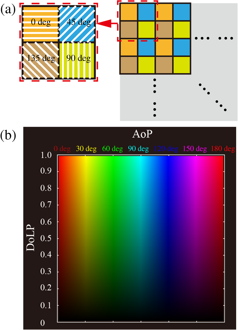

The degree of linear polarization (DoLP) and angle of polarization (AoP) can be obtained from the Stokes vector

Eq. (3)

DoLP = \sqrt{S_{1}^{2} + S_{2}^{2}} / S_{0},

Eq. (4)

AoP = (1 / 2) \tan^{- 1} (S_{2} / S_{1}) .

The three images for

S_{0}

, DoLP, and AoP can be fused into a single “polarization staining” image using the hue-saturation-intensity visualization scheme, which uses

S_{0}

for the brightness, AoP for hue, and DoLP for saturation.³³ In real applications, polarization staining with only DoLP and AoP generates satisfactory effects. The mapping strategy is shown as follows:

Eq. (5)

AoP \Rightarrow Hue, 100 % \Rightarrow Saturation, DoLP \Rightarrow Intensity .

This strategy takes advantage of the colorimetric representation as shown in Fig. 1(b) and is easy to identify by the human vision system. It avoids the influence of the light intensity variation and focuses on the visualization of polarization properties.

2.2.

Design of the Division of Focal Plane Polarimeter-Based 3 × 4 Mueller Matrix Microscope

The configuration of the DoFP polarimeter-based $3 \times 4$ Mueller matrix microscope is shown in Fig. 2. The original light source and the imaging sensor are replaced with the polarization states generator (PSG) and the DoFP polarimeter, respectively. In the PSG, the polarizer (Thorlabs) is fixed, thus no matter what SoP the light emitting diode (LED, Cree, 630 nm) irradiance is, the light passing through the polarizer will be linearly polarized with a constant light intensity. Measuring all columns of a Mueller matrix needs at least four illuminations with independent SoPs. The wave plate (Thorlabs) is rotated to four angles to produce the SoPs. For each illumination, the Stokes vector images of the specimen are calculated using the single-frame image of the DoFP polarimeter. The $i$ ’th ( $i = 1,2, 3$ , and 4) measurement is described as

Eq. (6)

S_{out} (i) = M_{sample} \cdot M_{W} \cdot M_{P} \cdot S_{LED},

where

M_{sample}

,

M_{W}

, and

M_{P}

are the Mueller matrices of the sample, the wave plate, and the polarizer, respectively.

S_{LED}

is the Stokes vector of the LED irradiance and

S_{out} (i)

is the Stokes vector of the specimen for the

i

’th illumination. If the polarizer is fixed to 0 deg, Eq. (6) can be expressed as

Eq. (7)

S_{out} (i) = M_{sample} \cdot S_{in} = M_{sample} \cdot [\begin{matrix} 1 \\ \cos^{2} 2 θ (i) + \sin^{2} 2 θ (i) \cos δ \\ 0.5 \sin 4 θ (i) (1 - \cos δ) \\ \sin 2 θ (i) \sin δ \end{matrix}],

where

δ

is the retardance of the wave plate and

θ (i)

is the

i

’th fast axis angle of the wave plate. The DoFP polarimeter records only the linear part of the Stokes parameters, hence only the first three rows of

M_{sample}

are measurable. Taking all the four Stokes vector measurements into account, the following equation can be obtained:

Eq. (8)

[S_{out}] = M_{sample} \cdot [S_{in}], [\begin{matrix} S_{0} (1) & S_{0} (2) & S_{0} (3) & S_{0} (4) \\ S_{1} (1) & S_{1} (2) & S_{1} (3) & S_{1} (4) \\ S_{2} (1) & S_{2} (2) & S_{2} (3) & S_{2} (4) \end{matrix}] = [\begin{matrix} m_{11} & m_{12} & m_{13} & m_{14} \\ m_{21} & m_{22} & m_{23} & m_{24} \\ m_{31} & m_{32} & m_{33} & m_{34} \end{matrix}] \times [\begin{matrix} 1 & \dots & 1 \\ \cos^{2} 2 θ (1) + \sin^{2} 2 θ (1) \cos δ & \dots & \cos^{2} 2 θ (4) + \sin^{2} 2 θ (4) \cos δ \\ 0.5 \sin 4 θ (1) (1 - \cos δ) & \dots & 0.5 \sin 4 θ (4) (1 - \cos δ) \\ \sin 2 θ (1) \sin δ & \dots & \sin 2 θ (4) \sin δ \end{matrix}] .

The Mueller matrix

M_{sample}

can then be calculated using

M_{sample} = [S_{out}] \times inv ([S_{in}])

, where inv (

[S_{in}]

) means the inverse of

[S_{in}]

. Here, the calculation of inv (

[S_{in}]

) is similar to that in Eq. (2). Since both

[S_{in}]

in Eq. (8) and the instrument matrix

A

in a complete rotating wave plate Stokes polarimeter are composed of a set of Stokes vectors, the minimum CN of [

S

] and

A

is equal. The CN of [

S_{in}

] should be minimized to reduce the errors transmitted from [

S_{out}

] to

M_{sample}

. When the retardance of the wave plate is 131.8 deg, the CN of [

S_{in}

] reaches to the minimum 1.732.³¹ However, a 131.8-deg wave plate is not commercially available and requires a custom order, which might influence the instrument’s accuracy. Thus, we adopt the commonly used quarter-wave plate and search the minimum CN of [

S_{in}

] using the genetic algorithm integrated in the MATLAB^® optimization toolbox. Calculation shows when the retardance of the wave plate is 90 deg, and the fast axes of the wave plate are set to (

- 51.69 \deg

,

- 15.12 \deg

, 15.12 deg, and 51.69 deg) or (

- 74.88 \deg

,

- 38.31 \deg

, 38.31 deg, and 74.88 deg), the CN of

[S_{in}]

reaches to the minimum 3.40. The above angle scheme yields four elliptical SoPs, which are not commonly used and studied. Thus, alternatively, we set two fast axes

θ (1)

and

θ (2)

to

- 45 \deg

and 45 deg to generate the left- and right-hand circularly polarized light, respectively, and optimize the remaining fast axes,

θ (3)

and

θ (4)

, by minimizing the CN of

[S_{in}]

. As shown in Fig. 3, when

θ (3) = 19.6 \deg

and

θ (4) = 160.4 \deg

(or

- 19.6 \deg

), the CN reaches to a local minimum 3.677, which is close to the optimal value 3.40. [Although the CN can reach 3.599 when

θ (3) = 15.9 \deg

and

θ (4) = 74.1 \deg

, we choose (

- 45 \deg

,

- 19.6 \deg

, 19.6 deg, and 45 deg) scheme for a faster measurement speed.]

Fig. 2

Photograph and configuration of the DoFP polarimeter-based $3 \times 4$ Mueller matrix microscope.

Fig. 3

CN map of $[S_{in}]$ . Color bar represents the common logarithm of the CN for better data visualization.

After the optimization of $[S_{in}]$ , the propagation of errors in Mueller matrix construction is minimized. However, for accurate measurement, the nonideal nature of the polarizing elements should be calibrated. The nonideal nature of the polarizing elements includes the rotation errors of the polarizer and the quarter-wave plate, and the retardance error of the quarter-wave plate. The calibration of the DoFP polarimeter-based Mueller matrix system includes the calibration of the DoFP polarimeter and calibration of the matrix $[S_{in}]$ . Because the DoFP polarimeter has already been calibrated, we only need to calibrate the matrix $[S_{in}]$ . When the sample is removed from the polarization microscope and the wave plate is rotated to four different angles ( $- 45 \deg$ , $- 19.6 \deg$ , 19.6 deg, and 45 deg), the first three rows of the matrix $[S_{in}]$ will be directly measured by the DoFP polarimeter, and the three errors can be calculated. The calibration shows that the real retardance of the quarter-wave plate used in this study is 90.98 deg. After the optimization and calibration of the matrix $[S_{in}]$ , the mean errors for all the Mueller matrix elements reach to about 0.3% and 0.6% when measuring the Mueller matrices of the air and a linear polarizer, respectively.

2.3.

Cancerous Tissue Samples

Cancer incidence is growing fast worldwide, making the pathological diagnoses of different cancer tissues crucial tasks. Using a conventional microscope, the features of carcinoma tissues are usually visible for stained slices but invisible for unstained ones. However, when observing the unstained slices using polarization imaging techniques, we can obtain abundant useful polarization information to distinguish the normal and abnormal tissues. To test the potential power of the DoFP polarimeter-based $3 \times 4$ Mueller matrix microscope, in this study, we apply it to human liver and cervical carcinoma tissue samples.

Figure 4 shows the carcinoma tissue slices provided and prepared by Shenzhen Sixth People’s Hospital. The slice shown in Fig. 4(a2) is a $4 - μ m$ thick hematoxylin–eosin (H–E) stained human liver carcinoma slice, and the slice shown in Fig. 4(a1) is the corresponding unstained, dewaxed $12 - μ m$ thick slice from the same biopsy sample archived in the hospital. The slice shown in Fig. 4(b2) is a $4 - μ m$ thick H–E stained human cervical carcinoma slice, and the slice shown in Fig. 4(b1) is the unstained, dewaxed $12 - μ m$ thick slice from the same biopsy sample. Because the two slices shown in Figs. 4(a1) and 4(a2) [and in Figs. 4(b1) and 4(b2)] are originally “twins” adjacent to each other, the cancerous areas should look similar. The microscopic images of the H–E stained slices are shown in Figs. 4(a3), 4(a4), 4(b3), and 4(b4). Many fibrous structures are visible across both slices, and the stained colors of the dysplastic regions are darker than that of healthy tissues. The microscopic images of the unstained, dewaxed $12 - μ m$ thick slices are shown in Figs. 6(a1) and 6(b1), respectively. From these images, we can see that the characteristic microstructures represented in the H–E stained slices are invisible in the unstained ones. This work was approved by the Ethics Committee of the Shenzhen Sixth People’s (Nanshan) Hospital.

Fig. 4

(a1) Unstained and (a2) H-E stained slices of the human liver carcinoma slice. (a3) and (a4) Microscopic images of the H-E stained human liver carcinoma slice. (b1) Unstained and (b2) H-E stained slices of the human cervical carcinoma slice. (b3) and (b4) Microscopic images of the H-E stained human cervical carcinoma slice. The developments of the liver cancer cells are often accompanied by inflammatory reactions and fibrosis formations in the surrounding tissues, whereas the cervical carcinoma processes usually lead to breaking down of the well-aligned structures existing in the healthy cervix tissues. The fibrosis structures are marked by dashed lines. The microstructures are visible in the H-E stained slices but invisible in the unstained slices. However, as shown in Figs. 5 and 6, the microstructures in the unstained slices are clearly visible using the polarization imaging method.

Fig. 5

The $3 \times 4$ Mueller matrix images of unstained human pathological specimens: (a) and (b) two regions on the liver carcinoma tissue slice and (c) and (d) two regions on the cervical carcinoma tissue slice. The Mueller matrix elements are all normalized by $m_{11}$ except $m_{11}$ . The color bar is from $- 1$ to 1 for $m_{11}$ , $m_{22}$ , and $m_{33}$ , and from $- 0.2$ to 0.2 for other elements for better image vision.

Fig. 6

(a1) and (b1) Intensity images and (a2) and (b2) polarization staining images of two regions on the unstained human liver carcinoma slices. (c1) and (d1) Intensity images and (c2) and (d2) polarization staining images of two regions on the unstained human cervical carcinoma slice. The colorimetric representation strategy is shown in Fig. 1(b). The brightness of the polarization staining image is increased with a factor of 5 for better image vision.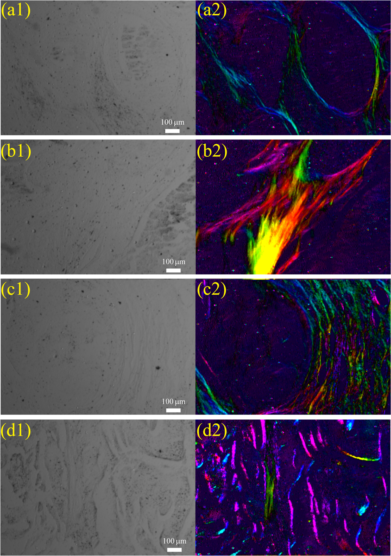

3. Results and Discussion

3.1.

3 × 4 Mueller Matrix Images of Unstained, Dewaxed Human Carcinoma Specimens

In order to test the potential diagnostic applications of the DoFP polarimeter-based polarization microscope, we measure the $3 \times 4$ Mueller matrix images of different regions of both the unstained, dewaxed $12 - μ m$ slices of human liver cancer specimen as shown in Figs. 6(a1) and 6(b1) and human cervical carcinoma specimen as shown in Figs. 6(c1) and 6(d1). Figures 5(a)–5(d) show the $3 \times 4$ Mueller matrix images of the unstained pathological samples. The fibrous structures can hardly be seen in the intensity images shown in Figs. 6(a1)–6(d1), but are significantly enhanced in the Mueller matrix images as shown in Fig. 5. Some previous studies have testified that the developments of the liver cancer cells are often accompanied by inflammatory reactions, leading to fibrosis formations in the surrounding tissues. During the pathological process from hepatitis to cirrhosis and liver cancer, the proportion of fibrous structures rises.²⁰ Therefore, the fibrosis degree can serve as a quantitative indicator for the detection and scoring of liver carcinoma tissues. It can be observed from the Mueller matrix elements shown in Fig. 5 that the proportion of fibrous structures in the area represented by Fig. 5(b) is higher than that represented by Fig. 5(a). On the other hand, the cervical carcinoma processes usually lead to breaking down of the well-aligned anisotropic structures in healthy cervix tissues, which can be used as diagnostic indicators from different cervical intraepithelial neoplasia stages to cervical cancer.²⁷ As indicated by the Mueller matrix elements shown in Fig. 5, the breakdown level of the well-aligned anisotropic structures in the area represented by Fig. 5(d) is higher than that represented by Fig. 5(c). It can be clearly observed from Fig. 5 that the intrinsic anisotropic fibrous structures of the cancerous liver and cervical tissues are mainly revealed in the $m_{24}$ and $m_{34}$ elements. Meanwhile, in other Mueller matrix elements, the microstructures are not significant or are even invisible, which are different from the characteristic features of Mueller matrices of bulk tissues measured in the reflection mode.⁷ When measuring a bulk tissue, the strong scattering power usually leads to a Mueller matrix with prominent patterns in all the elements. Hence, for the biomedical polarimetry in vivo, the $3 \times 3$ Mueller matrix imaging is appropriate. However, for the standard thin dewaxed human carcinoma tissue slices with limited scattering, the $3 \times 4$ Mueller matrix images can provide more important pathological information than linear polarized $3 \times 3$ Mueller matrix images.

The Mueller matrix can completely describe the polarization property of a specimen, but its physical meaning is not easy to understand. The diattenuation of a sample is a function of the first row of the Mueller matrix. For the thin carcinoma slice, the values of diattenuation are often very small. Since the diagonal $m_{11}$ , $m_{22}$ , and $m_{33}$ are close to one, we can safely assume that the samples are almost nondepolarizing. For the nondepolarizing samples, the linear retardance ( $δ$ ) and its orientation angle ( $θ$ ) can be derived as

Eq. (9)

δ = \sin^{- 1} (\sqrt{m_{24}^{2} + m_{34}^{2}} / m_{11}), θ = \frac{1}{2} \tan^{- 1} (\frac{- m_{24}}{m_{34}}) .

The value and orientation of the birefringence effect can be proven as potentially crucial information for pathologists. Since the tissue slices are usually very thin, their values of retardance are always small, resulting in more prominent values in the $m_{24}$ and $m_{34}$ than those in other elements. The small retardance is mostly induced by the microfibers in the tissue slices.¹⁹

3.2.

Single Shot “Polarization Staining” Using Circularly Polarized Light Illumination

From the Mueller matrix images in Fig. 5, we can conclude that the $m_{24}$ and $m_{34}$ elements containing important structural information may be useful for the diagnosis of some kinds of pathological tissues. For the ( $- 45 \deg$ , $- 19.6 \deg$ , 19.6 deg, and 45 deg) measurement scheme, when the fast axis of the wave plate is rotated to 45 deg and $- 45 \deg$ , the illumination light is right- and left-hand circularly polarized, respectively. For instance, under right-hand circularly polarized light illumination, the following equation can be obtained:

Eq. (10)

[\begin{matrix} S_{0} (4) \\ S_{1} (4) \\ S_{2} (4) \end{matrix}] = [\begin{matrix} m_{11} & m_{12} & m_{13} & m_{14} \\ m_{21} & m_{22} & m_{23} & m_{24} \\ m_{31} & m_{32} & m_{33} & m_{34} \end{matrix}] \cdot [\begin{matrix} 1 \\ 0 \\ 0 \\ 1 \end{matrix}] = [\begin{matrix} m_{11} + m_{14} \\ m_{21} + m_{24} \\ m_{31} + m_{34} \end{matrix}] .

Considering that the Mueller matrix elements $m_{14}$ , $m_{21}$ , and $m_{31}$ are close to zero as shown in Fig. 5, the following approximation can be obtained:

Eq. (11)

m_{11} \approx S_{0} (4), m_{24} \approx S_{1} (4), m_{34} \approx S_{2} (4) .

Thus, we can recast Eq. (9) as

Eq. (12)

δ = \sin^{- 1} [\sqrt{S_{1} {(4)}^{2} + S_{2} {(4)}^{2}}], θ = \frac{1}{2} \tan^{- 1} [\frac{- S_{1} (4)}{S_{2} (4)}] .

Equation (12) is similar to Eqs. (3) and (4). The information in

δ

and

θ

is essentially the same to those in DoLP and AoP. Thus, under right-hand circularly polarized light illumination, the polarization staining images of the unstained dewaxed human liver and cervical carcinoma specimens calculated using Eqs. (2)–(5) are shown in Figs. 6(a2)–6(d2), in which the information of

m_{24}

and

m_{34}

are encoded. Compared with the intensity images shown in Figs. 6(a1)–6(d1), the polarization staining images reveal much more detailed information of the microstructures, especially the pathological-related fibrosis with strong birefringence. The values of DoLP, as well as the color saturation of the polarization image of the fibrosis region, will be higher than the background. In addition to the value of the DoLP, the alignment orientations of the microfibers can also be clearly revealed from polarization staining images.

The color images of the H–E-stained slices and the polarization staining images of the unstained slices are based on different imaging contrast mechanisms. Therefore, the differences between the results shown in Fig. 4 and 6 are significant. Compared with Fig. 4, the anisotropic fibrosis structures in Fig. 6 are more prominent than other types of microstructures, meaning that the polarization imaging technique can be used to reveal the optical anisotropic nature of tissue samples in pathological assessments. The polarization staining imaging using circularly polarization light has several unique advantages: (a) many previous works have pointed out that the polarization imaging techniques are capable of providing additional structural information of the samples, especially information about structures smaller than the diffraction limit²⁶^–²⁸ and (b) the use of circularly polarized light illumination can avoid the orientation influence of the linearly or elliptically polarized light illuminations on the anisotropic microstructures widely existing in biological tissues.

Because both the intensity and the polarization staining images are obtained with single frames, using GPU acceleration algorithm, the DoFP polarimeter-based polarization microscope has the capacity for real-time polarization monitoring of dynamic processes such as living cell behaviors. Similarly, the use of the DoFP polarimeter and circularly polarized light illumination may make the implementation of the real-time polarization endoscope possible, too.

4. Conclusion

In this article, a DoFP polarimeter-based polarization microscope capable of simultaneously measuring both the Stokes vector and the $3 \times 4$ Mueller matrix with an optimal 4-SoP illumination is presented. We test the polarization microscope by measuring unstained human cancerous tissue slices. The experimental results show that the characteristic microstructures represented in the H–E-stained slices are invisible in the unstained ones. However, from the $3 \times 4$ Mueller matrix images, we can see that the fibrous structures are highlighted. The intrinsic anisotropic fibrous structures of the cancerous liver and cervical tissues are mainly revealed in the $m_{24}$ and $m_{34}$ elements. Meanwhile, in other Mueller matrix elements the microstructures are not significant or even invisible. The characteristic features of the $m_{24}$ and $m_{34}$ can be observed in the polarization staining images using the circularly polarized light as illumination. In this way, combined with GPU acceleration algorithm, the DoFP polarization microscope has the capacity for real-time polarization imaging of biomedical specimens to aid in clinical diagnosis.

Acknowledgments

This work has been supported by the National Natural Science Foundation of China Grant Nos. 11174178, 11374179, 61205199, and 61405102 and the Science and Technology Project of Shenzhen Grant Nos. CXZZ20140509172959978 and GJHZ20150316160614844.

References

1.

H. Ye et al., “On the circular birefringence of polycrystalline polymers: polylactide,” J. Am. Chem. Soc., 133 (35), 13848 –13851 (2011). http://dx.doi.org/10.1021/ja205159u JACSAT 0002-7863 Google Scholar

2.

S. Liu et al., “Mueller matrix imaging ellipsometry for nanostructure metrology,” Opt. Express, 23 (13), 17316 –17329 (2015). http://dx.doi.org/10.1364/OE.23.017316 OPEXFF 1094-4087 Google Scholar

3.

F. Snik et al., “An overview of polarimetric sensing techniques and technology with applications to different research fields,” Proc. SPIE, 9099 90990B (2014). http://dx.doi.org/10.1117/12.2053245 Google Scholar

4.

E. Namer, S. Shwartz and Y. Y. Schechner, “Skyless polarimetric calibration and visibility enhancement,” Opt. Express, 17 (2), 472 –493 (2009). http://dx.doi.org/10.1364/OE.17.000472 OPEXFF 1094-4087 Google Scholar

5.

S. Fang et al., “Image dehazing using polarization effects of objects and airlight,” Opt. Express, 22 (16), 19523 –19537 (2014). http://dx.doi.org/10.1364/OE.22.019523 OPEXFF 1094-4087 Google Scholar

6.

N. Ghosh and I. A. Vitkin, “Tissue polarimetry: concepts, challenges, applications, and outlook,” J. Biomed. Opt., 16 (11), 110801 (2011). http://dx.doi.org/10.1117/1.3652896 JBOPFO 1083-3668 Google Scholar

7.

S. Alali and A. Vitkin, “Polarized light imaging in biomedicine: emerging Mueller matrix methodologies for bulk tissue assessment,” J. Biomed. Opt., 20 (6), 061104 (2015). http://dx.doi.org/10.1117/1.JBO.20.6.061104 JBOPFO 1083-3668 Google Scholar

8.

B. Kunnen et al., “Application of circularly polarized light for non-invasive diagnosis of cancerous tissues and turbid tissue-like scattering media,” J. Biophotonics, 8 (4), 317 –323 (2015). http://dx.doi.org/10.1002/jbio.v8.4 Google Scholar

9.

R. S. Gurjar et al., “Imaging human epithelial properties with polarized light-scattering spectroscopy,” Nat. Med., 7 (11), 1245 –1248 (2001). http://dx.doi.org/10.1038/nm1101-1245 1078-8956 Google Scholar

10.

R. Weaver, “Rediscovering polarized light microscopy,” Am. Lab., 35 (20), 55 –61 (2003). Google Scholar

11.

R. Oldenbourg, “A new view on polarization microscopy,” Nature, 381 (27), 811 –812 (1996). http://dx.doi.org/10.1038/381811a0 Google Scholar

12.

O. Arteaga et al., “Mueller matrix microscope with a dual continuous rotating compensator setup and digital demodulation,” Appl. Opt., 53 (10), 2236 –2245 (2014). http://dx.doi.org/10.1364/AO.53.002236 APOPAI 0003-6935 Google Scholar

13.

Y. Liu et al., “Complementary fluorescence-polarization microscopy using division-of-focal-plane polarization imaging sensor,” J. Biomed. Opt., 17 (11), 116001 (2012). http://dx.doi.org/10.1117/1.JBO.17.11.116001 JBOPFO 1083-3668 Google Scholar

14.

V. Gruev, R. Perkins and T. York, “CCD polarization imaging sensor with aluminum nanowire optical filters,” Opt. Express, 18 (18), 19087 –19094 (2010). http://dx.doi.org/10.1364/OE.18.019087 OPEXFF 1094-4087 Google Scholar

15.

J. Millerd et al., “Pixelated phase-mask dynamic interferometer,” Proc. SPIE, 5531 304 –314 (2004). http://dx.doi.org/10.1117/12.560807 PSISDG 0277-786X Google Scholar

16.

W. Hsu et al., “Polarization microscope using a near infrared full-Stokes imaging polarimeter,” Opt. Express, 23 (4), 4357 –4368 (2015). http://dx.doi.org/10.1364/OE.23.004357 OPEXFF 1094-4087 Google Scholar

17.

S. L. Jacques, J. C. Ramella-Roman and K. Lee, “Imaging skin pathology with polarized light,” J. Biomed. Opt., 7 (3), 329 –340 (2002). http://dx.doi.org/10.1117/1.1484498 JBOPFO 1083-3668 Google Scholar

18.

E. Du et al., “Mueller matrix polarimetry for differentiating characteristic features of cancerous tissues,” J. Biomed. Opt., 19 (7), 076013 (2014). http://dx.doi.org/10.1117/1.JBO.19.7.076013 JBOPFO 1083-3668 Google Scholar

19.

M. Dubreuil et al., “Mueller matrix polarimetry for improved liver fibrosis diagnosis,” Opt. Lett., 37 (6), 1061 –1063 (2012). http://dx.doi.org/10.1364/OL.37.001061 OPLEDP 0146-9592 Google Scholar

20.

Y. Wang et al., “Differentiating characteristic microstructural features of canceroustissues using Mueller matrix microscope,” Micron, 79 8 –15 (2015). http://dx.doi.org/10.1016/j.micron.2015.07.014 MICNB2 0047-7206 Google Scholar

21.

L. Qiu et al., “Multispectral scanning during endoscopy guides biopsy of dysplasia in Barrett’s esophagus,” Nat. Med., 16 (5), 603 –606 (2010). http://dx.doi.org/10.1038/nm.2138 1078-8956 Google Scholar

22.

A. Pierangelo et al., “Multispectral Mueller polarimetric imaging detecting residual cancer and cancer regression after neoadjuvant treatment for colorectal carcinomas,” J. Biomed. Opt., 18 (4), 046014 (2013). http://dx.doi.org/10.1117/1.JBO.18.4.046014 JBOPFO 1083-3668 Google Scholar

23.

T. Novikova et al., “The origins of polarimetric image contrast between healthy and cancerous human colon tissue,” Appl. Phys. Lett., 102 241103 (2013). http://dx.doi.org/10.1063/1.4811414 APPLAB 0003-6951 Google Scholar

24.

A. Pierangelo et al., “Polarimetric imaging of uterine cervix: a case study,” Opt. Express, 21 (12), 14120 –14130 (2013). http://dx.doi.org/10.1364/OE.21.014120 OPEXFF 1094-4087 Google Scholar

25.

N. T. Clancy et al., “Polarised stereo endoscope and narrowband detection for minimal access surgery,” Biomed. Opt. Express, 5 (12), 4108 –4117 (2014). http://dx.doi.org/10.1364/BOE.5.004108 BOEICL 2156-7085 Google Scholar

26.

V. Sankaran, Jr. J. T. Walsh and D. J. Maitland, “Comparative study of polarized light propagation in biologic tissues,” J. Biomed. Opt., 7 (3), 300 –306 (2002). http://dx.doi.org/10.1117/1.1483318 JBOPFO 1083-3668 Google Scholar

27.

C. He et al., “Characterizing microstructures of cancerous tissues using multispectral transformed Mueller matrix polarization parameters,” Biomed. Opt. Express, 6 (8), 2934 –2945 (2015). http://dx.doi.org/10.1364/BOE.6.002934 BOEICL 2156-7085 Google Scholar

28.

P. G. Ellingsen et al., “Mueller matrix three-dimensional directional imaging of collagen fibers,” J. Biomed. Opt., 19 (2), 026002 (2014). http://dx.doi.org/10.1117/1.JBO.19.2.026002 JBOPFO 1083-3668 Google Scholar

29.

Z. Chen, X. Wang and R. Liang, “Calibration method of microgrid polarimeters with image interpolation,” Appl. Opt., 54 (5), 995 –1001 (2015). http://dx.doi.org/10.1364/AO.54.000995 APOPAI 0003-6935 Google Scholar

30.

R. Chipman, Handbook of Optics, I 3rd ed.McGraw-Hill, New York (2009). Google Scholar

31.

J. S. Tyo, “Design of optimal polarimeters: maximization of signal-to-noise ratio and minimization of systematic error,” Appl. Opt., 41 (1), 619 –630 (2002). http://dx.doi.org/10.1364/AO.41.000619 APOPAI 0003-6935 Google Scholar

32.

B. M. Ratliff, C. F. LaCasse and J. S. Tyo, “Interpolation strategies for reducing IFOV artifacts in microgrid polarimeter imagery,” Opt. Express, 17 (11), 9112 –9125 (2009). http://dx.doi.org/10.1364/OE.17.009112 OPEXFF 1094-4087 Google Scholar

33.

L. B. Wolff, “Polarization vision: a new sensory approach to image understanding,” Image Vision Comput., 15 81 –93 (1997). http://dx.doi.org/10.1016/S0262-8856(96)01123-7 IVCODK 0262-8856 Google Scholar

Biographies for the authors are not available.

CC BY: © The Authors. Published by SPIE under a Creative Commons Attribution 4.0 Unported License. Distribution or reproduction of this work in whole or in part requires full attribution of the original publication, including its DOI.

Citation Download Citation

Jintao Chang, Honghui He, Ye Wang, Yi Huang, Xianpeng Li, Chao He, Ran Liao, Nan Zeng, Shaoxiong Liu, and Hui Ma "Division of focal plane polarimeter-based 3 × 4 Mueller matrix microscope: a potential tool for quick diagnosis of human carcinoma tissues," Journal of Biomedical Optics 21(5), 056002 (9 May 2016). https://doi.org/10.1117/1.JBO.21.5.056002

Published: 9 May 2016

Access the abstract

JOURNAL ARTICLE
8 PAGES

DOWNLOAD PAPER SAVE TO MY LIBRARY

GET CITATION

CITATIONS

Cited by 65 scholarly publications and 1 patent.

Explore citations on Lens.org

KEYWORDS

Polarization

Polarimetry

Tissues

Microscopes

Wave plates

Liver

Calibration

1.

Introduction

2.

Methods and Materials

2.1.

Polarization Imaging Using the Division of Focal Plane Polarimeter

Eq. (1)

Eq. (2)

Fig. 1

Eq. (3)

Eq. (4)

Eq. (5)

2.2.

Design of the Division of Focal Plane Polarimeter-Based 3 × 4 Mueller Matrix Microscope

Eq. (6)

Eq. (7)

Eq. (8)

Fig. 2

Fig. 3

2.3.

Cancerous Tissue Samples

Fig. 4

Fig. 5

Fig. 6

3.

Results and Discussion

3.1.

3 × 4 Mueller Matrix Images of Unstained, Dewaxed Human Carcinoma Specimens

Eq. (9)

3.2.

Single Shot “Polarization Staining” Using Circularly Polarized Light Illumination

Eq. (10)

Eq. (11)

Eq. (12)

4.

Conclusion

Acknowledgments

References

Show All Keywords

Keywords/Phrases

Search In:

Publication Years