1.

Introduction

The emergence of nonlinear optics has led to tremendous improvements in optical microscopy. Different nonlinear optical microscopy (NOM) techniques, such as two-photon excitation fluorescence,^1,2 second-harmonic generation (SHG),^3–5 third-harmonic generation (THG),^6–11 nonlinear photothermal and photoacoustic,^12–14 and Raman scattering,^2,15,16 have been developed to overcome some drawbacks of linear optical microscopy.

NOM, in addition to increasing the resolution, has the ability to image deeper into the samples compared to linear optical microscopy when near-infrared (NIR) excitation is employed,^17–19 because using NIR excitation reduces the scattering and the optical absorption in biological systems. Scattering in samples leads to a background that reduces the signal-to-background ratio (SBR) and, as a result, blurs the deep images and decreases the resolution. Furthermore, using NIR becomes less likely to reduce the cell viability¹¹ as compared to shorter wavelengths, because of the reduced out-of-focus absorption.²⁰ Although exploiting longer wavelengths results in reduced scattering and generated background,¹⁸ the level of SBR is still low, which limits the maximum attainable imaging depth. On the other hand, in NOM, the signal is generated only in the regions with significant pump intensities, and, consequently, optical sectioning can take place when a tightly focused excitation laser beam is employed. However, despite the ability to overcome the diffraction-limited lateral resolution due to the nonlinearity of the imaging process,^12–14,21 the axial resolution in most of these techniques is not yet sufficient for optical sectioning in some applications. To enhance the axial resolution, a few techniques^22,23 have been reported; however, they suffer from various problems such as the need for multicolor pulses, complex and expensive setups, and/or being appropriate only for surface topography measurements.

To circumvent some of these drawbacks, we propose the modulation-detection technique or, in other words, derivative-detection technique. Its main advantage is phase-sensitive detection capability, which is used to limit the response of the detection system to a narrow interval centered at the modulation frequency. Furthermore, a frequency-independent background signal and background noise are essentially reduced, resulting in a higher signal-to-noise ratio, which makes this method superior to intensity-modulation techniques.²⁴ This method, while preserving all its advantages, can also be translated into spatial domain, where it can be implemented to point-scanning NOMs to boost their performance.

In this study, we introduce the focal-point axial modulation nonlinear optical microscopy (FPAM-NOM) and use it to improve THG microscopy using a single-color laser. We exploit its advantage to cancel out the background generated by turbid media surrounding the sample, to enhance the axial resolution and the localization, and also to resolve ambiguities in signal interpretation. Finally, since FPAM-NOM is based on the nonlinear optical properties of materials, it can be applied to label-free imaging for biological applications.

2.

Focal-Point Axial Modulation Nonlinear Optical Microscopy Principle

In FPAM-NOM, location of the focal point is modulated by a distance of $2{\delta }_0$ along the $z$-axis with a modulation frequency of $f$ [Figs. 1(a)–1(c)]. Consequently, the generated third-harmonic signal is also modulated, so that the THG signal before the detector in the cylindrical coordinate is

Fig. 1

Principle of FPAM-NOM and experimental setup. (a) Modulation of an interface inside the sample relative to the focal point along the axial direction with a modulation depth of $2{\delta }_0$. (b) Scanning the axial position of the modulating focal point along the $z$-direction relative to the interface-generated THG signal inside the sample. (c) Position of the interface relative to the focal point along the axial direction versus time. (d) Generated signal after lock-in amplifier versus the axial position of the interface relative to the focal point. The red vertical dashed lines represent the interface. (e) THG microscopy setup. In a conventional experiment, the chopper is on and the piezo-stage is off, while in the FPAM-NOM setup, the chopper is removed and the piezo-stage is on. In this study, ${\delta }_0=1\mu \mathrm{m}$, and frequencies of the chopper and the function generator are 249.3.

In principle, THG is more significant when the interfaces of the sample under study are located within one confocal parameter from the focal plane,²¹ which itself provides some inherent sectioning.^8,14 However, in conventional THG microscopy, interpretation of the signal comes with some ambiguities. That is because it is not clear whether any change in the level of the signal is related to the variation of the axial distance of the interface from focus in negative or positive $z$-direction, or it comes from a possible variation of the material properties. But in FPAM technique, the sign of $S_f(z)$ changes when the focus traverses the interface [Fig. 1(d)], and, hence, the location of the sectioning plane (focal plane) and also the $z$-direction of the interface can be precisely determined. Consequently, by comparison of the data obtained from the two methods (conventional and FPAM), one can conclude whether the change in the detected signal is due to the variation in the material property or the interface-sectioning plane distance. Furthermore, as the FPAM signal [Fig. 1(d)] varies linearly as a function of $z$ around the interface ($\mathrm{\Delta }z=0$), it could be used for optical sectioning and localization.^25,26

3.

Materials and Methods

3.2.

Image Formation

The third-harmonic images are synthesized through point-by-point measurement with the sample scanned by a stepper motor stage with 25-nm resolution (Melles Griot, NanoMax-HS). THG images of the red blood cell (RBC) are acquired by the $XYZ$ stepper motor stage scanned with step sizes of $1\mu \mathrm{m}$ along the $z$-axis and step sizes of 200 nm along the $x$- and $y$-axes. In this setup, the laser beam enters from the bottom and the PMT is located on top of the sample. Hence, in scanning along the $z$-axis, moving toward the laser leads to more negative $z$. Therefore, the left peak in Figs. 2(a), 2(g), and 2(h) corresponds to the coverslip’s side toward the PMT and far from the laser (deeper within the sample).

Fig. 2

Conventional and FPAM-NOM THG microscopy signals of axially scanned samples. (a) THG microscopy signal of a coverslip using conventional (dashed line) and FPAM-NOM (solid line) setups. Gray area shows the coverslip. THG image of a wedge with (b) conventional and (c) FPAM-NOM methods. Raw data in place of the maximum resolving limits of (d) the former and (f) the later techniques correspond to blue and red dashed lines in (b) and (c), respectively. (e) A point between the two maximum resolving limits of the two methods. THG generated from a thin layer of baked egg-white sandwiched between two coverslips using (g) conventional and (h) FPAM-NOM techniques. The principle of background cancellation (i) in only turbid media and (j) the numerical reconstruction of it in the media including baked egg-white sandwiched between two coverslips corresponding to (h). The vertical dashed lines in (d)–(f) illustrate the glass–oil interfaces acquired from corresponding 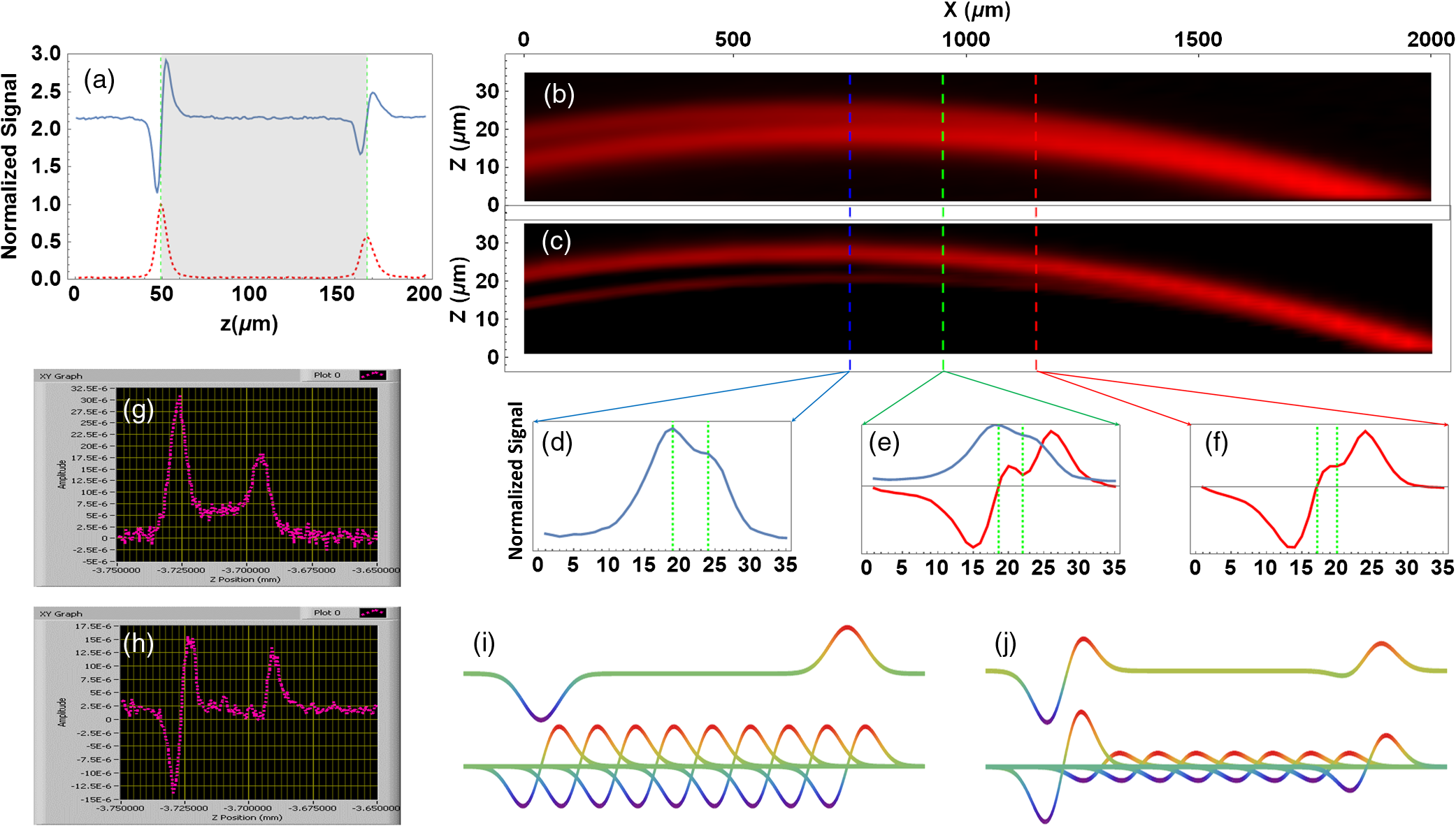data.

4.

Results and Discussion

Figure 2(a) shows the signals acquired by conventional (dashed line) and FPAM-THG (solid line) techniques from glass–air interfaces by scanning a coverslip along its surface normal. As is evident, FPAM-NOM signal (solid line) is proportional to the first derivative of the signal of the conventional setup (dashed line) with respect to $z$. The two peaks with $120\text{-}\mu \mathrm{m}$ distance correspond to the surfaces of the coverslip.

To verify the axial-resolution enhancement by FPAM-NOM, the images from the $xz$ plane of a wedge are taken using conventional [Fig. 2(b)] and FPAM-NOM [Fig. 2(c)] techniques. Figures 2(d) and 2(f) show the corresponding detected signal profiles along the left and the right dashed lines in Figs. 2(b) and 2(c), respectively. They represent the maximum resolving limits of conventional and FPAM-NOM techniques, respectively. Figure 2(e) shows the detected signal for the central dashed line to compare the acquired signal by the two techniques for a point located between the two maximum resolution limits. The best axial resolutions achieved using conventional and FPAM-NOM methods are 5 and $2.8\mu \mathrm{m}$, respectively, which shows an enhancement of about 1.8 times. We expect further improvement of the axial resolution and the enhancement factor using, respectively, objectives with higher numerical aperture and higher harmonic detection modes of the lock-in amplifier.²⁴

Another interesting advantage of FPAM-NOM, which originates from its derivative nature, occurs in imaging of a sample within a turbid medium, such as a brain, in which the distance between the interfaces of its components (e.g., cell dendrites and organelles) is shorter than the axial resolving power. In such media, imaging by a conventional technique generates a significant level of signal from the surrounding media [Fig. 2(g)]. This signal acts as a background, blurring the sample edges. Employing FPAM-NOM eliminates such background and generates high-contrast images [Fig. 2(h)]. To verify this, a thin layer of baked egg-white (turbid medium) sandwiched between two coverslips (sample) is used and scanned along the $z$-axis.

As is evident, in FPAM-NOM, unlike the conventional setup [Fig. 2(g)], the THG signal from the egg-white layer (the background signal) is eliminated from the detected signal, and accordingly, the interfaces of the coverslips become more visible, and SBR increases as well [Fig. 2(h)]. The achieved peak of the SBR enhancement factor, here, is about 25.3. Note that this background is the signal generated by the turbid media and cannot be canceled by nonderivative techniques. The reason of such enhancement can be explained as follows: the egg-white layer can be considered as a stack of infinitely thin slabs, each generating a THG signal. In normal NOM method, they add up and contribute to the background signal. However, in FPAM-NOM, the THG signals generated from the adjacent slabs cancel out each other. Such cancellation is due to the derivative nature of those signals [Fig. 2(i)], and, therefore, no background from the turbid media is observed in the signal. By this explanation, we can interpret the signal in Fig. 2(h) as a superposition of the signals from the two glass/egg-white interfaces and that from the turbid media, which is numerically reconstructed and is shown in Fig. 2(j). It is interesting to note that although the right peak (deeper sample interface) is less intense than the left one, its SBR enhancement factor is bigger (25.3 against 20.1), which implies that the depth-dependent signal attenuation is less pronounced in FPAM as compared to a conventional method.

Finally, to show the localization enhancement and resolving ambiguities by FPAM, the images of an RBC are acquired and compared with that acquired by conventional THG microscopy. As can be seen in Fig. 3, while the conventional images cannot resolve the axial displacement of $4\mu \mathrm{m}$ among the four frames [Figs. 3(a)–3(d)], the FPAM technique can well resolve the sample points, which are below (blue) or above (red) the scanning plane [Figs. 3(e)–3(h)]. Hence, as the scanning plane moves toward the top of the cell, the blue region increases and the size of the red area reduces. The image also shows that the RBC is placed obliquely relative to the coverslip surface [Figs. 3(e)–3(h)], which is difficult, or even impossible, to be recognized with most other techniques.

Fig. 3

THG images of an RBC. Normalized $x-y$ frames of (a)–(d) conventional and (e)–(h) FPAM-NOM techniques. The blue area shows the sample interfaces below the scanning plane, while the red area represents those above it. For convenience, the blue and red regions were individually normalized. All frames have $1\mu \mathrm{m}$ of axial distance from each other. For convenience, the intersections of the sample with the scanning planes are illustrated by white. Scale bar: $1\mu \mathrm{m}$.

Such features of FPAM-NOM result in better resolved images with sharper edges from samples inside turbid media, which makes it advantageous for applications such as brain imaging. Furthermore, one can use the signals before and after the lock-in amplifier to benefit from the advantages of conventional and FPAM techniques simultaneously. Finally, although this report is dedicated to THG microscopy, FPAM-NOM is also applicable to some other NOMs, e.g., SHG.