Fast direct reconstruction strategy of dynamic fluorescence molecular tomography using graphics processing units

Maomao Chen; Jiulou Zhang; Chuangjian Cai; Yang Gao; Jianwen Luo

doi:10.1117/1.JBO.21.6.066010

14 June 2016 Fast direct reconstruction strategy of dynamic fluorescence molecular tomography using graphics processing units

Maomao Chen, Jiulou Zhang, Chuangjian Cai, Yang Gao, Jianwen Luo

Author Affiliations +

Journal of Biomedical Optics, Vol. 21, Issue 6, 066010 (June 2016). https://doi.org/10.1117/1.JBO.21.6.066010

Abstract

Dynamic fluorescence molecular tomography (DFMT) is a valuable method to evaluate the metabolic process of contrast agents in different organs in vivo, and direct reconstruction methods can improve the temporal resolution of DFMT. However, challenges still remain due to the large time consumption of the direct reconstruction methods. An acceleration strategy using graphics processing units (GPU) is presented. The procedure of conjugate gradient optimization in the direct reconstruction method is programmed using the compute unified device architecture and then accelerated on GPU. Numerical simulations and in vivo experiments are performed to validate the feasibility of the strategy. The results demonstrate that, compared with the traditional method, the proposed strategy can reduce the time consumption by ∼90% without a degradation of quality.

1. Introduction

As a rapidly developing technique for pharmacokinetics studies,¹^,² dynamic fluorescence imaging reflects the absorption, distribution, and excretion characteristics of contrast agents in the body. The reconstructed pharmacokinetic images of dynamic fluorescence molecular tomography (DFMT) can provide noninvasive and three-dimensional (3-D) monitoring of the metabolic process of fluorophores in vivo.³^–⁵ Therefore, it is promising for tumor detection, drug development, and metabolic research.⁶^,⁷

Generally, two kinds of methods can be used to solve DFMT problems: indirect methods and direct methods. Indirect methods³ have been developed from the conventional static fluorescence molecular tomography (FMT) procedures. It is assumed that the concentration of the fluorophores is constant during the data acquisition process of each circle. Therefore, the individual FMT image of each circle is reconstructed first, and then the metabolic parameters of each voxel can be obtained with curve fitting. Some methods have been previously proposed for FMT reconstruction. L2 regularization⁸ is commonly implemented because it is simple and can be efficiently solved, while L1-based regularization⁹^,¹⁰ can improve the resolution of the reconstruction images especially for spars problems. However, the spatial resolution and accuracy of the images obtained with the indirect methods are relatively low because the static assumption is not suitable for the DFMT problems, especially when the concentration of the fluorophores varies fast over time. To overcome this problem, direct reconstruction methods⁴^,⁵ have been proposed to map the metabolic parameters into the acquired datasets and directly reconstruct the dynamic images from the boundary measurements in one step. By using the direct methods, the quality of the reconstructed images is improved. However, the time consumption of the direct methods is significantly increased. In a typical DFMT implementation with about 10,000 boundary measurement points, 5000 finite-element nodes, and 200 iterations, the direct methods take more than 8 h to obtain the reconstructed images.

Some methods can be used to accelerate the direct methods. Principal components analysis (PCA) has been proposed to reduce the dimension of weight matrix.¹¹ Wavelet¹²^,¹³ and Fourier¹⁴ transforms have been employed to reduce the scale of the boundary measurements. However, these methods may reduce the accuracy of the reconstructed images due to the information lost by using data compression.

Parallel computation using graphics processing units (GPU) is a fast-developing technology. The computing ability of GPU is much more powerful than that of general-purpose central processing units (CPU). Combined with deeply optimized processing pipelines, hierarchical thread structures and extremely low memory latency, GPU constitutes an excellent shared memory parallel computing platform.¹⁵ However, programming on GPU had been difficult until the compute unified device architecture (CUDA) was introduced in 2006. CUDA is a parallel computing platform and programming model and provides a software environment where developers can use a high-level programming language, such as C. CUDA-enabled GPU has been utilized in the field of fluorescence imaging, such as the acceleration of Monte Carlo algorithm,¹⁵ modeling of time-resolved photon migration,¹⁶ and acceleration of early-photon FMT.¹⁷

In this work, a fast computing strategy using GPU is proposed to accelerate the direct reconstruction algorithm of DFMT. In this strategy, the most time-consuming part of the algorithm, i.e., iterative regularization using conjugate gradient (CG) optimization, is accelerated using CUDA. Meanwhile, to fully use the parallel computing ability of GPU, vectors of fluorophore concentration are assembled into a distribution matrix according to the order of the projection sequences in each circle. Then the forward prediction measurements are calculated in the form of matrix–matrix multiplication.

Numerical simulations and in vivo mouse experiments are carried out to evaluate the performance of the proposed strategy. The results demonstrate that the proposed strategy can significantly accelerate the direct DFMT algorithm almost without any quality degradation.

2. Method

2.1.

Data Acquisition System

A hybrid FMT/x-ray computed tomography (XCT) system¹⁸ is used to obtain the DFMT boundary measurements. As shown in Fig. 1, a free-space and full-angle FMT system is used to acquire the fluorescence datasets, while an XCT system is used to obtain the anatomical information of the small animal, which provides structural priors for the reconstruction algorithm. For dynamic FMT problems, to monitor the metabolic process of the fluorophores, the small animal is fixed on the stage and continuously rotated for $K$ circles, and the charge-coupled device (CCD) camera acquires $S$ projections in each circle. Therefore, a total of $P = K S$ projections are obtained during the whole DFMT acquisition process.

Fig. 1

Schematic of the hybrid FMT/XCT system. The FMT system is used to acquire the DFMT measurements, while the XCT system obtains the anatomical information of the small animal.

2.2.

Direct Reconstruction Method for Dynamic Fluorescence Molecular Tomography Problems

For FMT problems, the propagation of the excitation and emission light in biological tissues can be reasonably approximated by two coupled diffusion equations.¹⁹^,²⁰ Using Green’s function theory, the fluorescence signal $Φ_{m} (r_{d}, r_{s})$ detected at a point $r_{d}$ due to a excitation source at $r_{s}$ can be written as²¹

Eq. (1)

Φ_{m} (r_{d}, r_{s}) = Θ \int G_{m} (r_{d}, r) n (r) G_{x} (r, r_{s}) d^{3} r,

where the Green’s function

G_{x} (r, r_{s})

stands for the light propagation from the source point

r_{s}

to an arbitrary position

r

inside the medium at the excitation wavelength

x

. The Green’s function

G_{m} (r_{d}, r)

describes the light propagation from a position

r

inside the medium to the detector point

r_{d}

at the emission wavelength

m

, and

n (r)

denotes the fluorescent yield to be reconstructed.

In DFMT problems, a two-compartment model is commonly used to describe the metabolic process of the fluorophores inside different organs.²² The concentration of fluorophores $n (r, t)$ at time $t$ can be obtained using²³

Eq. (2)

n (r, t) = - A (r) \exp [- α (r) t] + B (r) \exp [- β (r) t],

where

A (r)

and

B (r)

determine the zero-time concentration at position

r

,

α (r)

, and

β (r)

denote the uptake and excretion rates of the fluorophores.²³

When the imaged 3-D volume is discretized into $N$ voxels, the parametric images in the discrete domain can be defined as

Eq. (3)

X = [x_{1}, x_{2}, x_{3}, x_{4}] = [A, B, α, β],

where each parametric image

x_{u} (u = 1,2, 3,4)

is given by

x_{u} = {[x_{u} (r_{1}), \dots, x_{u} (r_{N})]}^{T}

, and

r_{j} (j = 1, \dots, N)

is employed to denote the spatial locations of voxels in the discretized domain.

As demonstrated in Sec. 2.1, the measurement acquisition consists of $K$ circles, and $S$ projections are performed in each circle. For projection $s (s = 1, \dots, s)$ , the surface of the imaged object is orthographically projected to the fluorescence image, which is obtained from CCD camera. The CCD pixels inside the projection area are considered to be the measurement points, and the number of the measurement points is $M_{s}$ . Thus, a total of $P = K S$ projections and $M = \sum_{s = 1}^{s} M_{s}$ measurement points are obtained. Let $t_{p} = (p = 1, \dots, P)$ denote the individual discrete time of projections. By combining Eqs. (1) and (2), the pharmacokinetic parameters can be mapped directly to the boundary measurements as follows:⁴

Eq. (4)

Φ_{m} (r_{d_{i}}, K S_{s}, t_{p}) = \sum_{j = 1}^{N} W_{s} (i, j) n (r_{j}, t_{p}) = \sum_{j = 1}^{N} W_{s} (i, j) {- A (r_{j}) \exp [- α (r_{j}) t_{p}] + B (r_{j}) \exp [- β (r_{j}) t_{p}]},

where

W_{s}

is the submatrix of the weight matrix

W

at projection

s (s = 1, \dots, S)

, and its entries are defined as²⁴

Eq. (5)

W_{s} (i, j) = Δ V Θ G_{m} (r_{d_{i}}, r_{j}) G_{x} (r_{j}, K S_{s}),

where is the volume of each individual voxel.

Let $f (X)$ denote the forward model. The boundary measurements predicted by the forward model is given as

Eq. (6)

f (X, t_{p}) = [Φ_{m} (r_{d_{i}}, K S_{s}, t_{p}), \dots, Φ_{m} (r_{d_{M_{s}}}, K S_{s}, t_{p})],

Eq. (7)

f (X) = {[f {(X, t_{1})}^{T}, \dots, f {(X, t_{P})}^{T}]}^{T} .

To reconstruct the parametric images in one step, by combining Eq. (7) and the conventional Tikhonov regularization method, a new objective function is obtained for the direct reconstruction method⁵

Eq. (8)

Ψ (X) = {‖ y - f (X) ‖}_{2}^{2} + λ_{1} {‖ L A ‖}_{2}^{2} + λ_{2} {‖ L B ‖}_{2}^{2} + λ_{3} {‖ L α ‖}_{2}^{2} + λ_{4} {‖ L β ‖}_{2}^{2} = {‖ y - f (X) ‖}_{2}^{2} + \sum_{u = 1}^{4} {‖ L x_{u} ‖}_{2}^{2},

where

y = {[y {(t_{1})}^{T}, y {(t_{2})}^{T}, \dots, y {(t_{p})}^{T}]}^{T}

denotes the whole boundary measurement matrix assembled using measurement vectors of all the frames.

λ_{u} (u = 1,2, 3,4)

is the regularization parameter, and

L

is the Laplacian-type regularization matrix²⁵ constructed using the structural priors obtained with the XCT system. The minimization of

Ψ (X)

can be solved using a CG scheme.²⁶

2.3.

Proposed Graphics Processing Units Acceleration Strategy

2.3.1.

Flow chart of the acceleration strategy

The flow chart of the direct reconstruction method and the acceleration strategy are shown in Fig. 2. The entire procedure of the algorithm consists mainly of three parts, i.e., the construction of Laplacian-type regularization matrix²⁵ (part 1 in Fig. 2), the low dimensional estimation of the initial of parameters²⁷ (part 2 in Fig. 2), and the CG optimization (part 3 in Fig. 2). The most important and time-consuming part is the CG optimization. In the CG optimization, four dynamic parameters ( $A$ , $B$ , $α$ , and $β$ ) are iteratively optimized until the end conditions are satisfied. The iteration number of the CG optimization is usually set to be more than 100, and the iterations take more than 99% of the whole reconstruction time. Therefore, the CG optimization needs to be accelerated.

Fig. 2

Flowchart of the acceleration strategy. The whole procedure of CG optimization (part 3) is programmed and accelerated using CUDA.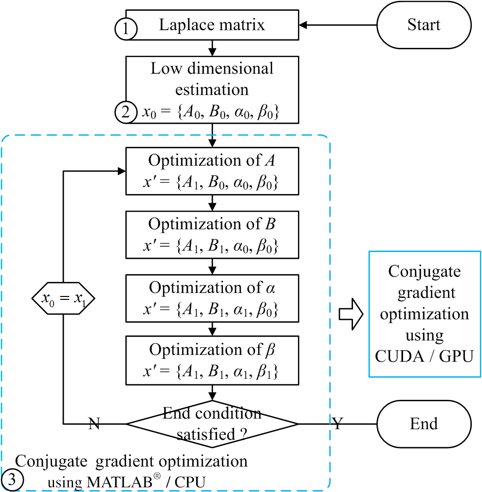

As shown in Fig. 2, the whole procedure of the optimization is programmed using CUDA, while the rest parts of the algorithm are programmed in MATLAB^® 2012 (The MathWorks, Inc., Natick, Massachusetts). For each metabolic parameter, the gradient $g [Ψ (x)]$ and the conjugate searching direction $d [ψ (X)]$ of the objective function $ψ (X)$ as shown in Eq. (8) are first calculated, and then the optimal step length is determined using golden search. These steps are all parallel computed using GPU. All the datasets and parameters are transferred to and stored in GPU memories before the GC scheme is started, and the reconstructed results are read out after it is finished. The whole optimization procedure is independently and automatically operated in GPU. This design can avoid frequent data transfer between CPU and GPU, which is significantly time-consuming especially when the size of the dataset is large.

2.3.2.

Parallel computing strategy

CUDA is a parallel computing platform and programming model invented by NVIDIA Corp. (Santa Clara, California). It is capable of sending C codes straight to GPU without complicated manipulation of the underlying GPU hardware. When using CUDA, the parallel computing functions are programmed as kernel functions, which could be operated on a GPU. However, it requires a lot of practice and experience to develop high-effective kernel functions. To solve this problem, NVIDIA provides a cuBLAS library, which is a high-effective implementation of basic linear algebra subprograms (BLAS).

In this study, the GPU method is programmed using CUDA C, and compiled using nvcc and mex compilers. The generated mex file can be invoked by MATLAB^® program. Some basic linear algebra calculations, such as matrix–matrix multiplication/addition, matrix–vector multiplication, and vector–vector dot product, are programmed using cuBLAS libraries. Take matrix–matrix multiplication for example, a parallelly tiled multiplication method is used in cuBLAS library. The diagram of the tiled multiplication is shown in Fig. 3(a). The matrixes $A$ , $B$ and $C = A \times B$ are divided into several submatrixes. When calculating the submatrix $C_{sub} = A_{sub} \times B_{sub}$ , the submatrixes $A_{sub}$ and $B_{sub}$ are synchronously read into the shared memories, and the elements are multiplied and accumulated parallelly in GPU threads. The block size of the submatrixes is selected based on the number of the GPU cores and the size of the GPU shared memories. The block size is set to be 16 in this study, and the number of elements for each submatrix is $16 \times 16 = 256$ .

Fig. 3

Diagram of the parallel computing strategy. (a) Diagram of the tiled multiplication method for matrix–matrix multiplication. The matrixes are divided into submatrixes, and the elements of the submatrixes are parallelly calculated. (b) Diagram of the parallel computing for the exponential value of the vector. The vector is divided into $N_{d}$ blocks, and each block contains $N_{t}$ threa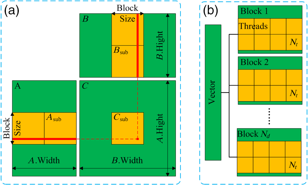ds.

For the functions that the cuBLAS cannot support, self-defined kernel functions are used to realize parallel computing. For example, when calculating the exponential values of a vector, the vector of size $N_{v}$ is divided into $N_{d}$ blocks, and each block contains $N_{t}$ GPU threads, as shown in Fig. 3(b). In this study, the threads number of each block is 512. Therefore, the vector is divided into $N_{d} = N_{v} / 512$ blocks. For each block, 512 elements of the vector are read synchronously to the shared memory, and the exponential values of the elements are calculated parallelly in the GPU threads.

2.3.3.

Predicted boundary measurements acceleration

The CG optimization is composed of gradient calculation and golden search. During the process of golden search, the predicted boundary measurements $f (X)$ in Eq. (7) are calculated repeatedly to minimize the objective function $Ψ (X)$ in Eq. (8). As shown in Fig. 3, $K$ circles and $S$ projections per circle are acquired in the measurements, $n_{s, k} (s = 1, \dots, S; k = 1, \dots, K)$ is the $N \times 1$ fluorophore concentration distribution vector at the $s$ ’th projection in the $k$ ’th circle, and $W_{s}$ is the submatrix with a size of $M_{s} \times N$ . Thus, one predicted boundary measurement $f (X)$ needs $K S$ matrix–vector multiplications. In a typical implementation, calculation of $f (X)$ is repeated over 7000 times, which takes more than 70% of the total reconstruction time.

Note that in Fig. 4(a), the concentration distribution vectors at the $s$ ’th projection in different circles share the same submatrix $W_{s}$ . To fully utilize the advantage of parallel computation of CUDA, the $K S$ fluorophore vectors are assembled to $S$ fluorophore matrixes with a size of $N \times K$ according to the sequence order of the submatrix $W_{s}$ . Therefore, $K S$ matrix–vector multiplications are transformed into $S$ matrix–matrix multiplications as shown in Fig. 4(b).

Fig. 4

Schematic of the predicted boundary measurements acceleration strategy. (a) The traditional method requires $K S$ matrix–vector multiplications to obtain the predicted boundary measurements. (b) The acceleration strategy assembles the fluorophore vectors to $S$ matrixes and requires only $S$ matrix–matrix multiplications to obtain the predicted boundary measurements.

2.4.

Comparison Principal Components Analysis Acceleration Method

PCA is a widely used method to accelerate the reconstructions of FMT problems by reducing the dimensions of the measurement datasets and the weight matrixes.¹¹ It linearly transforms an original set of variables into a substantially smaller set of uncorrelated variables, which can represent most of the information in the original set of variables. The cumulative percent of variance (CPV) is used to determine the number of retained principal components.¹¹ An appropriate CPV should be carefully selected to balance the calculation speed and the reconstruction accuracy.

For FMT problems, the optimal CPV can be reasonably set to be about 0.9 according to the previous study.¹¹ However, for DFMT problems, the optimal CPVs vary dramatically among different experimental cases. To obtain a proper balance between the time consumption and the reconstruction quality, the CPVs for the numerical simulations and the in vivo experiments are empirically selected to be 0.7 and 0.995, respectively.

2.5.

Evaluation Method

The time consumptions of the traditional method, the proposed GPU method, and the PCA method are compared and the acceleration ratios are calculated. The relative difference (RD) is calculated to evaluate the differences between the results reconstructed by the acceleration methods and the traditional method, and it is defined as¹¹^,¹³^,¹⁷

Eq. (9)

R D = s q r t (‖ X_{fast} - X_{traditional} ‖ / X_{traditional}),

where

X_{traditional}

is the entire 3-D parametric images reconstructed using the traditional method.

X_{fast}

denotes the 3-D reconstruction results obtained from the GPU- or PCA-based acceleration method.

The traditional method, the proposed GPU acceleration strategy, and the PCA acceleration method are all performed in MATLAB^® 2012 (The MathWorks, Inc., Natick, Massachusetts) on a PC workstation with Intel^® Core™ i7-4770 CPU at 3.40 GHz and 12 GB RAM. The PC workstation is embedded with an NVDIA GTX 750 Ti graphics card with 640 CUDA cores and 2 GB video memories.

3. Experiments and Results

3.1.

Numerical Simulations

3.1.1.

Simulation setups

Numerical simulations are performed to validate the performance of the acceleration strategy. A Digimouse atlas²⁸ shown in Fig. 5(a) is employed to construct a 3-D simulation model, which includes four kinds of organs: heart, lungs, liver, and kidneys. Different optical properties are assigned to these organs to constitute a heterogeneous model, as presented in Table 1.²⁹ The Digimouse model is discretized into $N$ mesh voxels using COMSOL Multiphysics 3.5 (COMSOL Inc., Stockholm, Sweden).

Fig. 5

Numerical simulations. (a) The 3-D Digimouse model used in the simulations. The mouse torso from the neck to the bottom of the kidneys is selected as the investigated region, with a total length of 3.1 cm. (b) ICG concentration curves simulating the metabolic process of ICG in different organs.

Table 1

Optical properties and pharmacokinetic parameters setups in different regions.

Regions	μa (cm−1)	μs′ (cm−1)	A (a.u.)	B (a.u.)	α (min−1)	β (min−1)
Heart	0.350	23	1.7	1.7	0.330	0.023
Liver	0.500	13	1.0	1.0	0.435	0.011
Lungs	0.250	30	0.8	0.8	0.296	0.020
Kidneys	0.175	20	1.2	1.2	0.254	0.016
Background	0.300	10	0.5	0.5	0.348	0.009

Figure 5(b) shows indocyanine green (ICG) concentration curves, which simulate the metabolic processes of ICG in different organs and tissues. The curves are obtained according to Eq. (2), and the corresponding pharmacokinetic parameters are listed in Table 1.⁵

In the simulations, the atlas model is suspended on a rotation stage and continuously rotated for 60 circles. Each circle takes 1 min and acquires 24 projections with an angular increment of 15 deg. During the process of the measurement, the ICG concentrations of different organs vary in each projection according to the metabolic curves shown in Fig. 5(b).

Two parameters determine the size of the datasets and the time consumption of the reconstruction, i.e., the number of the discretized voxels $N$ and the number of the boundary measurements $M$ . Two groups of datasets are made to evaluate the effect of these two parameters on the reconstruction speed, and each group contained four cases. In group one, $M$ is constant and $N$ varies in different cases, while in group two, $N$ is constant and $M$ varies. The parameter setup in each case is listed in Table 2. To compare with the GPU method, the PCA method is implemented to reduce the size of the measurements $M$ , and the compression threshold $CPV s$ are set to be 0.7 for all the simulation cases.

Table 2

Original and PCA compressed data sizes for simulations.

	Voxels N	Measurements M		Compression ratio
	Voxels N	Original	PCA	Compression ratio
Group 1
Case 1	5651	15,620	2229	7.0
Case 2	6968	15,620	1933	8.0
Case 3	9096	15,620	1440	10.8
Case 4	12,768	15,620	1030	15.2
Group 2
Case 5	10,793	7730	696	11.1
Case 6	10,793	9443	803	11.8
Case 7	10,793	11,476	997	11.5
Case 8	10,793	12,861	1047	12.2
Average				10.9

3.1.2.

Simulation results

The original and the PCA compressed data sizes of the numerical simulations are listed in Table 2. For the eight simulation cases, the original data sizes of the measurements range from 7730 to 15,620, while the compressed data sizes are between 696 and 2229. The maximum and minimum compression ratios are 7.0 and 15.2, respectively. According to the results, using PCA compression, the data sizes of the measurements are reduced on average to about 10% of the original data sizes.

The time consumptions of the traditional, GPU, and PCA methods are listed in Table 3, and the acceleration ratios are calculated. The time consumption of the traditional method ranges between 18,135 and 42,448 s, which is considered to be too long, especially when the reconstruction is operated repeatedly to obtain the optimal regularization parameters. The time costs of the GPU method are between 1485 and 3646 s, while the time costs of the PCA method are between 2861 and 4176. The average acceleration ratios of the GPU and PCA methods are 12.2 and 7.9, respectively. It indicates that the acceleration performance of the GPU method is better than the PCA method.

Table 3

Time consumptions and acceleration ratios of the GPU and PCA methods for simulations.

	Time (s)			Acceleration ratio
	Traditional	GPU	PCA	GPU	PCA
Group 1
Case 1	22,135	1485	2861	14.9	7.7
Case 2	25,996	1867	3032	13.9	8.6
Case 3	33,225	2491	3453	13.3	9.6
Case 4	42,448	3646	4176	11.6	10.2
Group 2
Case 5	18,135	1826	3393	9.9	5.3
Case 6	22,057	2060	3498	10.7	6.3
Case 7	26,557	2343	3654	11.3	7.3
Case 8	29,682	2566	3708	11.6	8.0
Average				12.2	7.9

The $RD s$ of the parametric images obtained from the GPU and PCA methods are listed in Table 4. The maximum average RD for the GPU and PCA methods are 0.013 and 0.031, respectively. According to the results demonstrated in Tables 3 and 4, a comparison can be made between the GPU and PCA methods for the numerical simulations. When the CPV value is set to be 0.7, the computational speed of the GPU method is faster than that of the PCA method, while the reconstruction quality of the GPU method is better than that of the PCA method.

Table 4

RDs of the results obtained with the GPU and PCA methods for simulations.

	GPU				PCA
	A	B	α	β	A	B	α	β
Group 1
Case 1	0.003	0.002	0.003	0.002	0.038	0.003	0.006	0.003
Case 2	0.009	0.001	0.002	0.001	0.020	0.003	0.021	0.003
Case 3	0.053	0.003	0.012	0.004	0.048	0.002	0.013	0.003
Case 4	0.011	0.003	0.003	0.004	0.042	0.002	0.007	0.004
Group 2
Case 5	0.017	0.002	0.011	0.001	0.047	0.003	0.014	0.003
Case 6	0.003	0.003	0.013	0.002	0.031	0.003	0.014	0.006
Case 7	0.005	0.002	0.008	0.003	0.013	0.001	0.006	0.002
Case 8	0.004	0.001	0.008	0.001	0.009	0.002	0.007	0.003
Average	0.013	0.002	0.008	0.002	0.031	0.003	0.011	0.003

Figure 6 shows the cross-sectional images of the reconstruction results obtained by the traditional, GPU, and PCA methods in simulation case 4, and the images are taken from the liver region of the Digimouse corresponding to the red dashed line in Fig. 5(a). Figure 7 shows the cross-sectional images in the kidney region corresponding to the black dashed line in Fig. 5(a). There are no obvious differences between the reconstructed results. The same findings can be obtained in all other cases in the simulations (not shown).

Fig. 6

Cross-sectional parametric images for simulation case 4 in the region of liver corresponding to the red dashed line in Fig. 5(a). (a)–(d) The results reconstructed with the traditional method. (e)–(h) The results reconstructed with the GPU method. (i)–(l) The results reconstructed with the PCA method.

Fig. 7

Cross-sectional parametric images for simulation case 4 in the region of kidneys corresponding to the black dashed line in Fig. 5(a). (a)–(d) The results reconstructed with the traditional method. (e)–(h) The results reconstructed with the GPU method. (i)–(l) The results reconstructed with the PCA method.

3.2.

In Vivo Experiment

3.2.1.

Experimental setups

In vivo experiments are conducted based on a hybrid FMT/XCT system described in Sec. 2.1. A 300 W Xenon lamp (MAX-302, Asahi Spectra, Torrance, California) is employed as the excitation source. A fiber is attached to the lamp to generate a line-shaped excitation source with a length of 4 cm. The excitation light is filtered through a $770 \pm 6 - nm$ bandpass excitation filter (XBPA770, Asahi Spectra, Torrance, California), and the power density of the excitation light is $0.03 mW / {cm}^{2}$ . On the opposite side of the excitation source, the emitted ICG fluorescence is filtered with an $840 \pm 6 - nm$ bandpass emission filter (FF01-840/12-25, Semrock, Rochester, New York) and detected by a $512 \times 512 pixel$ , $- 70 ° C$ cooled CCD camera (iXon DU-897, Andor Technologies, Belfast, Northern Ireland, United Kingdoms). The exposure time of the CCD camera is 1 s, and the CCD binning is set to be $512 \times 512$ .

A healthy BALB/c nude mouse with an age of about 8 weeks is fixed on the rotation stage and anesthetized. A bolus of ICG (0.1 mL, $50 μ g / mL$ ) is injected via the tail vain. During the DFMT measurements acquisition, the mouse is continuously rotated for 50 circles ( $K = 50$ ) with an angular increment of 15 deg. Therefore, 24 projections ( $S = 24$ ) are obtained in each circle, and a total of 1200 projections ( $P = K S = 50 \times 244$ ) are acquired for the entire DFMT measurement.

After the fluorescence data acquisition is finished, a hepatobiliary contrast agent for XCT imaging, Fenestra LC (Advanced Research Technologies, Montreal, California), is injected at a dose of $15 mL / kg$ body weight through the tail vein. One hour after the injection, the XCT images are collected to provide structural prior information. The x-ray tube works at 45 kVp and 1 mA during the scan, and the XCT images are collected by a complementary metal oxide semiconductor flat-panel detector (C7921-02, Hamamatsu, Japan).

In the mouse experiments, a total of 12,968 measurements are acquired. As shown in Fig. 8(a), a chest region with a height of 2.5 cm of the mouse is used to reconstruct the parametric images, and the reconstructed region is discretized into 6062 voxels. The transversal XCT images indicated by the green and red dashed lines in Fig. 8(a) are shown in Figs. 8(b) and 8(c). The XCT images are manually segmented into four regions: liver, lungs, kidneys, and the background. The Laplacian-type²⁵ regularization matrix is constructed according to the segmentation results. Figures 8(d) and 8(e) depict the segmented results corresponding to Figs. 8(b) and 8(c). The structural priors are used to create a heterogeneous model by assigning different optical properties to relevant regions, as shown in Table 1. Additionally, the PCA-based acceleration method is compared with the proposed GPU method, and the CPV is set to 0.995.

Fig. 8

XCT results of the mouse experiments. (a) Coronal XCT image in the chest region of the mouse. (b) and (c) Transversal XCT images indicated by the green and red dashed lines in (a), respectively. (d) and (e) Manually segmented organs corresponding to (b) and (c).

3.2.2.

Experimental results

As shown in Table 5, the number of the measurements $M$ is reduced from 12,968 to 2507 with PCA, and the compression ratio is about five times. The time consumptions of the traditional, GPU, and PCA methods are listed in Table 6. The acceleration ratios of the GPU and PCA methods are 9.8 and 9.4, respectively. The acceleration performances of the GPU and PCA methods are very close.

Table 5

Original and PCA compressed data sizes for the mouse experiments.

Voxels N	Measurements M		Compression ratio
Voxels N	Original	PCA	Compression ratio
6062	12,968	2507	5.2

Table 6

Time consumptions and acceleration ratios of the GPU and PCA methods for the mouse experiments.

Time(s)			Acceleration ratio
Traditional	GPU	PCA	GPU	PCA
32,512	3326	3466	9.8	9.4

The $RD s$ obtained with the GPU and PCA methods are shown in Table 7. The RDs of four parameters reconstructed with the PCA method are all larger than those with the GPU method. With a CPV value of 0.995, the reconstruction quality of the GPU method is better than PCA, while the acceleration performances of these two methods are close.

Table 7

RDs of the results obtained with the GPU and PCA methods for the mouse experiments.

	A	B	α	β
GPU	0.018	0.009	0.010	0.012
PCA	0.053	0.035	0.021	0.027

The cross-sectional parametric images obtained with the traditional, GPU, and PCA methods for the mouse experiments are shown in Fig. 9, and the images are taken from the lung region of the mouse corresponding to the red dashed line in Fig. 8(a). Figure 10 shows the cross-sectional images in the kidney region of the mouse corresponding to the green dashed line in Fig. 8(a). For all the reconstruction images, no visual differences can be observed.

Fig. 9

Cross-sectional parametric images for the mouse experiments in the region of lung corresponding to the red dashed line in Fig. 8(a). (a)–(d) The results reconstructed with the traditional method. (e)–(h) The results reconstructed with the GPU method. (i)–(l) The results reconstructed with the PCA method.

Fig. 10

Cross-sectional parametric images for the mouse experiments in the region of kidneys corresponding to the green dashed line in Fig. 8(a). (a)–(d) The results reconstructed with the traditional method. (e)–(h) The results reconstructed with the GPU method. (i)–(l) The results reconstructed with the PCA method.

4. Discussions

DFMT is a promising technique that can be used in tumor detection, drug development, and metabolic research.³ The previously proposed direct reconstruction method can improve the quality of the DFMT result.⁵ However, the implementation of the direct reconstruction method is limited due to the large time consumption. Generally, several hours are needed to reconstruct the DFMT images. Therefore, it is necessary to accelerate the direct method.

In this study, an acceleration strategy using GPU for DFMT is presented. The results of the numerical simulations and in vivo experiments demonstrate that this strategy can efficiently reduce the time cost of the reconstruction, with nearly no quality degradation.

As previously mentioned, the performances of the GPU and PCA methods are compared. For the GPU method, an appropriate CPV should be carefully selected to balance the calculation speed and the reconstruction accuracy.¹¹ A smaller CPV achieves faster computational speed, while a larger CPV obtains better reconstruction quality. In addition, the selection of CPV also depends on the specific data used. In this paper, the CPV was empirically selected to be 0.7 and 0.995 in the simulations and in vivo experiments, respectively. The GPU method does not need such a data-dependent parameter, and it may be convenient to use once it is implemented. On the other hand, information is lost to some extent in the PCA method, which could reduce the quality of the reconstruction results, especially when the CPV is set to be too small. On the contrary, all the measurement information can be retained when using the GPU method.

Furthermore, the PCA- and GPU-based methods are two different approaches to acceleration of FMT reconstruction and can be combined together to further increase the computational speed. Simulation case 1 is used to study the performance of the combination of the PCA and GPU methods, and the CPV is set to be 0.7. The time consumption of the combination method is 452 s, i.e., the acceleration ratio is increased to 48.9. The maximum RD is 0.043, which is slightly larger than that of the PCA method (0.038). The results demonstrate that, by combining the PCA and GPU methods, the computational speed can be significantly improved, and the loss of the image quality is acceptable.

5. Conclusion

In conclusion, the direct DFMT reconstruction algorithm is accelerated using a GPU-based strategy. The feasibility of this method is confirmed by numerical simulations and in vivo experiments. According to the results, the time consumptions are reduced to $\sim 10 %$ of the traditional method. The average RD of simulations and in vivo experiments is less than 2%, which means the errors between the acceleration method and the traditional method are negligible.

Acknowledgments

This work was supported by the National Natural Science Foundation of China under Grant Nos. 81227901, 81271617, 61322101, and 61361160418; and the National Major Scientific Instrument and Equipment Development Project under Grant No. 2011YQ030114. All applicable international, national, and/or institutional guidelines for the care and use of animals were followed. All procedures performed in studies involving animals were in accordance with the ethical standards of the Ethics Committee of Tsinghua University. This article does not contain any studies with human participants performed by any of the authors.

References

1.

M. Gurfinkel et al., “Pharmacokinetics of ICG and HPPH-car for the detection of normal and tumor tissue using fluorescence, near-infrared reflectance imaging: a case study,” Photochem. Photobiol., 72 (1), 94 –102 (2000). http://dx.doi.org/10.1562/0031-8655(2000)0720094POIAHC2.0.CO2 PHCBAP 0031-8655 Google Scholar

2.

E. M. C. Hillman and A. Moore, “All-optical anatomical co-registration for molecular imaging of small animals using dynamic contrast,” Nat. Photonics, 1 (9), 526 –530 (2007). http://dx.doi.org/10.1038/nphoton.2007.146 Google Scholar

3.

G. Zhang et al., “Imaging of pharmacokinetic rates of indocyanine green in mouse liver with a hybrid fluorescence molecular tomography/x-ray computed tomography system,” J. Biomed. Opt., 18 (4), 040505 (2013). http://dx.doi.org/10.1117/1.JBO.18.4.040505 Google Scholar

4.

G. L. Zhang et al., “A direct method with structural priors for imaging pharmacokinetic parameters in dynamic fluorescence molecular tomography,” IEEE Trans. Biomed. Eng., 61 (3), 986 –990 (2014). http://dx.doi.org/10.1109/TBME.2013.2292714 Google Scholar

5.

G. L. Zhang et al., “Full-direct method for imaging pharmacokinetic parameters in dynamic fluorescence molecular tomography,” Appl. Phys. Lett., 106 (8), 081110 (2015). http://dx.doi.org/10.1063/1.4913690 Google Scholar

6.

A. B. Milstein, K. J. Webb and C. A. Bouman, “Estimation of kinetic model parameters in fluorescence optical diffusion tomography,” J. Opt. Soc. Am. A., 22 (7), 1357 –1368 (2005). http://dx.doi.org/10.1364/JOSAA.22.001357 Google Scholar

7.

A. Alacam and B. Yazici, “Direct reconstruction of pharmacokinetic-rate images of optical fluorophores from NIR measurements,” IEEE Trans. Med. Imaging, 28 (9), 1337 –1353 (2009). http://dx.doi.org/10.1109/TMI.2009.2015294 Google Scholar

8.

X. Cao et al., “An adaptive Tikhonov regularization method for fluorescence molecular tomography,” Med. Biol. Eng. Comput., 51 (8), 849 –858 (2013). http://dx.doi.org/10.1007/s11517-013-1054-5 Google Scholar

9.

J. Dutta et al., “Joint L-1 and total variation regularization for fluorescence molecular tomography,” Phys. Med. Biol., 57 (6), 1459 –1476 (2012). http://dx.doi.org/10.1088/0031-9155/57/6/1459 Google Scholar

10.

J. J. Yu et al., “Sparse reconstruction for fluorescence molecular tomography via a fast iterative algorithm,” J. Innov. Opt. Health Sci., 7 (3), 1450008 (2014). http://dx.doi.org/10.1142/S1793545814500084 Google Scholar

11.

X. Cao et al., “Accelerated image reconstruction in fluorescence molecular tomography using dimension reduction,” Biomed. Opt. Express, 4 (1), 1 –14 (2013). http://dx.doi.org/10.1364/BOE.4.000001 Google Scholar

12.

T. J. Rudge, V. Y. Soloviev and S. R. Arridge, “Fast image reconstruction in fluoresence optical tomography using data compression,” Opt. Lett., 35 (5), 763 –765 (2010). http://dx.doi.org/10.1364/OL.35.000763 OPLEDP 0146-9592 Google Scholar

13.

T. Correia et al., “Wavelet-based data and solution compression for efficient image reconstruction in fluorescence diffuse optical tomography,” J. Biomed. Opt., 18 (8), 086008 (2013). http://dx.doi.org/10.1117/1.JBO.18.8.086008 Google Scholar

14.

J. Ripoll, “Hybrid Fourier-real space method for diffuse optical tomography,” Opt. Lett., 35 (5), 688 –690 (2010). http://dx.doi.org/10.1364/OL.35.000688 Google Scholar

15.

Q. Q. Fang and D. A. Boas, “Monte Carlo simulation of photon migration in 3D Turbid media accelerated by graphics processing units,” Opt. Express, 17 (22), 20178 –20190 (2009). http://dx.doi.org/10.1364/OE.17.020178 Google Scholar

16.

B. Zhang et al., “The CUBLAS and CULA based GPU acceleration of adaptive finite element framework for bioluminescence tomography,” Opt. Express, 18 (19), 20201 –20214 (2010). http://dx.doi.org/10.1364/OE.18.020201 Google Scholar

17.

X. Wang et al., “Acceleration of early-photon fluorescence molecular tomography with graphics processing units,” Comput. Math. Methods Med., 2013 297291 (2013). http://dx.doi.org/10.1155/2013/297291 Google Scholar

18.

X. L. Guo et al., “A combined fluorescence and microcomputed tomography system for small animal imaging,” IEEE Trans. Biomed. Eng., 57 (12), 2876 –2883 (2010). http://dx.doi.org/10.1109/TBME.2010.2073468 Google Scholar

19.

A. B. Milstein et al., “Fluorescence optical diffusion tomography,” Appl. Opt., 42 (16), 3081 –3094 (2003). http://dx.doi.org/10.1364/AO.42.003081 Google Scholar

20.

A. Joshi, W. Bangerth and E. M. Sevick-Muraca, “Adaptive finite element based tomography for fluorescence optical imaging in tissue,” Opt. Express, 12 (22), 5402 –5417 (2004). http://dx.doi.org/10.1364/OPEX.12.005402 Google Scholar

21.

M. A. O’Leary et al., “Fluorescence lifetime imaging in turbid media,” Opt. Lett., 21 (2), 158 –160 (1996). http://dx.doi.org/10.1364/OL.21.000158 Google Scholar

22.

D. J. Cuccia et al., “In vivo quantification of optical contrast agent dynamics in rat tumors by use of diffuse optical spectroscopy with magnetic resonance imaging coregistration,” Appl. Opt., 42 (16), 2940 –2950 (2003). http://dx.doi.org/10.1364/AO.42.002940 Google Scholar

23.

H. Shinohara et al., “Direct measurement of hepatic indocyanine green clearance with near-infrared spectroscopy: separate evaluation of uptake and removal,” Hepatology, 23 (1), 137 –144 (1996). http://dx.doi.org/10.1002/hep.510230119 HEPADF 0161-0538 Google Scholar

24.

D. Hyde et al., “A statistical approach to inverting the born ratio,” IEEE Trans. Med. Imaging, 26 (7), 893 –905 (2007). http://dx.doi.org/10.1109/TMI.2007.895467 Google Scholar

25.

S. C. Davis et al., “Image-guided diffuse optical fluorescence tomography implemented with Laplacian-type regularization,” Opt. Express, 15 (7), 4066 –4082 (2007). http://dx.doi.org/10.1364/OE.15.004066 Google Scholar

26.

S. R. Arridge and M. Schweiger, “A gradient-based optimisation scheme for optical tomography,” Opt. Express, 2 (6), 213 –226 (1998). http://dx.doi.org/10.1364/OE.2.000213 Google Scholar

27.

A. Brooksby et al., “Near-infrared (NIR) tomography breast image reconstruction with a priori structural information from MRI: algorithm development for reconstructing heterogeneities,” IEEE J. Sel. Top. Quantum, 9 (2), 199 –209 (2003). http://dx.doi.org/10.1109/JSTQE.2003.813304 Google Scholar

28.

B. Dogdas et al., “Digimouse: a 3D whole body mouse atlas from CT and cryosection data,” Phys. Med. Biol., 52 (3), 577 –587 (2007). http://dx.doi.org/10.1088/0031-9155/52/3/003 Google Scholar

29.

D. Hyde et al., “Performance dependence of hybrid x-ray computed tomography/fluorescence molecular tomography on the optical forward problem,” J. Opt. Soc. Am. A, 26 (4), 919 –923 (2009). http://dx.doi.org/10.1364/JOSAA.26.000919 Google Scholar

Biography

Maomao Chen received his bachelor’s and master’s degrees in biomedical engineering from Chongqing University in 2006 and 2009, respectively. Currently, he is a PhD candidate in the Department of Biomedical Engineering, Tsinghua University. His research interest is fluorescence molecular tomography for small animal imaging.

Jiulou Zhang is a PhD candidate in the Department of Biomedical Engineering, Tsinghua University, Beijing, China. His research interest is fluorescence molecular tomography for small animal imaging.

Chuangjian Cai received his bachelor’s degree in biomedical engineering, Tsinghua University, Beijing, China, in 2015. Currently, he is a PhD candidate in the Department of Biomedical Engineering, Tsinghua University. His research interest is fluorescence molecular tomography for small animal imaging.

Yang Gao received his bachelor’s degree in pharmaceutical sciences from Tsinghua University, Beijing, China, in 2014. Currently, he is a PhD candidate in the Department of Biomedical Engineering, Tsinghua University. His research interest is fluorescence molecular imaging.

Jianwen Luo is a professor at Tsinghua University. He was enrolled in the Thousand Young Talents Program in 2012 and received the Excellent Young Scientists Fund from the National Natural Science Foundation of China in 2013. He serves as an advisory editorial board member of the Journal of Ultrasound in Medicine, associate editor of Medical Physics, and faculty member of Faculty of 1000. His research interest is biomedical imaging, including ultrasound imaging and fluorescence molecular imaging.

Citation Download Citation

Maomao Chen, Jiulou Zhang, Chuangjian Cai, Yang Gao, and Jianwen Luo "Fast direct reconstruction strategy of dynamic fluorescence molecular tomography using graphics processing units," Journal of Biomedical Optics 21(6), 066010 (14 June 2016). https://doi.org/10.1117/1.JBO.21.6.066010

Published: 14 June 2016

Access the abstract

JOURNAL ARTICLE
11 PAGES

DOWNLOAD PAPER SAVE TO MY LIBRARY

GET CITATION

CITATIONS

Cited by 4 scholarly publications.

Explore citations on Lens.org

RIGHTS & PERMISSIONS

Get copyright permission Get copyright permission on Copyright Marketplace

KEYWORDS

Principal component analysis

Luminescence

Fluorescence tomography

Tomography

In vivo imaging

Reconstruction algorithms

Graphics processing units

1.

Introduction

2.

Method

2.1.

Data Acquisition System

Fig. 1

2.2.

Direct Reconstruction Method for Dynamic Fluorescence Molecular Tomography Problems

Eq. (1)

Eq. (2)

Eq. (3)

Eq. (4)

Eq. (5)

Eq. (6)

Eq. (7)

Eq. (8)

2.3.

Proposed Graphics Processing Units Acceleration Strategy

2.3.1.

Flow chart of the acceleration strategy

Fig. 2

2.3.2.

Parallel computing strategy

Fig. 3

2.3.3.

Predicted boundary measurements acceleration

Fig. 4

2.4.

Comparison Principal Components Analysis Acceleration Method

2.5.

Evaluation Method

Eq. (9)

3.

Experiments and Results

3.1.

Numerical Simulations

3.1.1.

Simulation setups

Fig. 5

Table 1

Table 2

3.1.2.

Simulation results

Table 3

Table 4

Fig. 6

Fig. 7

3.2.

In Vivo Experiment

3.2.1.

Experimental setups

Fig. 8

3.2.2.

Experimental results

Table 5

Table 6

Table 7

Fig. 9

Fig. 10

4.

Discussions

5.

Conclusion

Acknowledgments

References

Biography

Show All Keywords

Keywords/Phrases

Search In:

Publication Years