Reproducibility of parameters of postocclusive reactive hyperemia measured by diffuse optical tomography

Ernesto E. Vidal-Rosas; Stephen A. Billings; Timothy J. Chico M.D.; Daniel Coca

doi:10.1117/1.JBO.21.6.066012

15 June 2016 Reproducibility of parameters of postocclusive reactive hyperemia measured by diffuse optical tomography

Ernesto E. Vidal-Rosas, Stephen A. Billings, Timothy J. Chico M.D., Daniel Coca

Author Affiliations +

Journal of Biomedical Optics, Vol. 21, Issue 6, 066012 (June 2016). https://doi.org/10.1117/1.JBO.21.6.066012

Abstract

The application of near-infrared spectroscopy (NIRS) to assess microvascular function has shown promising results. An important limitation when using a single source-detector pair, however, is the lack of depth sensitivity. Diffuse optical tomography (DOT) overcomes this limitation using an array of sources and detectors that allow the reconstruction of volumetric hemodynamic changes. This study compares the key parameters of postocclusive reactive hyperemia measured in the forearm using standard NIRS and DOT. We show that while the mean parameter values are similar for the two techniques, DOT achieves much better reproducibility, as measured by the intraclass correlation coefficient (ICC). We show that DOT achieves high reproducibility for muscle oxygen consumption (ICC: 0.99), time to maximal HbO₂ (ICC: 0.94), maximal HbO₂ (ICC: 0.99), and time to maximal HbT (ICC: 0.99). Absolute reproducibility as measured by the standard error of measurement is consistently smaller and close to zero (ideal value) across all parameters measured by DOT compared to NIRS. We conclude that DOT provides a more robust characterization of the reactive hyperemic response and show how the availability of volumetric hemodynamic changes allows the identification of areas of temporal consistency, which could help characterize more precisely the microvasculature.

1. Introduction

Atherosclerosis and resulting cardiovascular diseases such as stroke and myocardial infarction are a major cause of death in developed countries. These account for more than 32% of mortality worldwide,¹ and in England and Wales cardiovascular disease was responsible for almost 30% of deaths in 2011.² Many noninvasive methods have been developed to assess the peripheral vascular system and identify signs of atherosclerosis at an early stage. Optical methods, in particular, have received attention due to their capability of measuring tissue oxygenation and blood perfusion³^,⁴ and because they offer several attractive features, such as portability, compactness, fast data acquisition, and noninvasiveness.

Near-infrared spectroscopy (NIRS) can determine changes in tissue hemodynamics and oxygenation⁵^,⁶ by measuring tissue absorbance at several wavelengths in the near-infrared range of the electromagnetic spectrum (650 to 950 nm). Typically, NIRS employs a few source-detector pairs to carry out measurements. As a consequence, the spatial resolution of NIRS, which is dictated by the optode separation, is relatively low.⁷ Diffuse optical tomography (DOT) overcomes this limitation by employing a larger number of sources and detectors to enable three-dimensional (3-D) volumetric reconstruction⁸ of changes in tissue hemodynamics.

NIRS and DOT have been used in a wide range of applications including functional imaging of the brain,⁹ assessment of muscle oxygenation,¹⁰ and cancer detection. It is widely accepted that DOT outperforms NIRS.⁸^,¹¹ For example, localized changes in hemodynamics due to motor tasks in adults and motor-sensory brain activation in neonates were accurately measured using DOT, while NIRS could not even detect relative changes¹¹ because of low spatial sampling. In another study, DOT could discriminate the somatosensory activation of two fingers, while in the same experiment, a 12-channel NIRS setting failed to resolve the activation.¹² Among the factors affecting the accuracy of NIRS concentration calculations are the differences in the pathlength factor: location, spatial extent, and heterogeneous distribution of absorption changes, e.g., multiple absorption foci. Although these sources of error could be minimized,¹³ DOT accounts for these problems implicitly.⁷

DOT requires solving two distinct problems: the forward problem and the inverse problem. The forward problem requires solving of the equation governing the photon transport in tissue to predict the detector measurements; typically this involves solving a diffusion equation over a 3-D spatial domain using the finite element method. The inverse problem involves estimating the optical properties of tissue to minimize the difference between experimental and model-predicted measurements; this is achieved by solving a nonlinear optimization problem, which can take hours to complete even on a high-end workstation. However, as we have recently demonstrated,¹⁴ it is possible to significantly speed up reconstruction of hemodynamic changes in complex tissue structures by using reduced order models of photon transport in tissue. This makes it possible to perform real-time monitoring of hemodynamic responses even with relatively modest computing resources.

NIRS, like other methods of measuring microvascular function, can detect significant differences in microvascular function between groups of healthy controls and patients with peripheral vascular diseases,¹⁵^–¹⁷ peripheral artery disease (PAD), and coronary heart disease.¹⁷^–¹⁹ However, these techniques are highly variable and have not been shown to be helpful in predicting an individual’s risk of future cardiovascular disease. Therefore, from a clinical point of view, refinements that improve reproducibility and reduce variability are highly desirable.

Typically, the evaluation of microvascular function by NIRS relies solely on a few measuring channels, and although repeatability and accuracy of results are promising,¹⁸^,²⁰^,²¹ there has not been a direct comparison of the parameters obtained during and after arterial occlusion by NIRS versus DOT. Furthermore, while multichannel systems for analysis of microvascular function are available,²²^–²⁵ studies on repeatability are lacking.

This study aims to evaluate and compare, using experimental data collected from healthy volunteers, the intrasubject reproducibility of key parameters of the hemodynamic response during postocclusive reactive hyperemia, obtained using DOT and NIRS, and to highlight the potential advantages of DOT in assessing endothelial function.

2. Methods

2.1.

Subjects

This study was approved by the Research Ethics Committee of the University of Sheffield. A group of 17 subjects was recruited, after giving informed consent. The group consisted of 11 men and 6 women. Baseline characteristics are listed in Table 1. Smokers or those with a history of cardiovascular disease were excluded.

Table 1

Baseline characteristic of study subjects (n=17).

Characteristic	Values
Age (year)	$33 \pm 7.5$
Weight (kg)	$70.5 \pm 14.1$
Height (cm)	$172.1 \pm 8.3$
BMI ( $kg / m^{2}$ )	$23.6 \pm 3.4$
Smokers	0

It is known that measurement of vascular function is greatly influenced by external factors such as recent activity, diet, time of day, and so on. These influences greatly reduce the applicability of vascular function measurement to clinical practice since in the real world it is difficult or impossible to control these factors. For this reason, we did not ask participants to fast or refrain from physical activity or caffeine for either of their visits.

2.2.

Instrumentation

DOT and NIRS measurements were obtained using a dynamic near-infrared optical tomography (DYNOT) instrument (NIRx). The system illuminates the tissue with four laser diodes at wavelengths $λ = 725$ , 760, 810, and 830 nm.

The diodes are modulated at distinct frequencies and then coupled with 30, 1 mm multimode optical fibers—optodes—acting both as sources and detectors. Synchronous detection allows parallel measurement at a sampling frequency of 1.8 Hz.²⁶ The optodes were organized in a hexagonal pattern with an interoptode spacing of 8 mm as shown in Fig. 1(a) and placed in a solid plastic holder to avoid movement artifacts [Fig. 1(b)]. For simplicity, hemoglobin concentration was calculated using only the wavelengths at 760 and 830 nm, chosen based on their symmetry with respect to the isobestic point of the extinction coefficients of hemoglobin.

Fig. 1

Experimental setup for NIRS and DOT measurement of reactive hyperemia. (a) Array with 30 optodes placed 8 mm apart in a hexagonal pattern. Optodes in red were used for NIRS measurements. All optodes were used for DOT reconstructions. (b) Placement of optode array on volar forearm of subject. (c) Rectangular finite element mesh used to model forearm tissue with dimensions $92 mm \times 35 mm \times 24 mm$ ( $W \times L \times D$ ). Blue circles at $z = 0 mm$ indicate the location of the 30 optodes.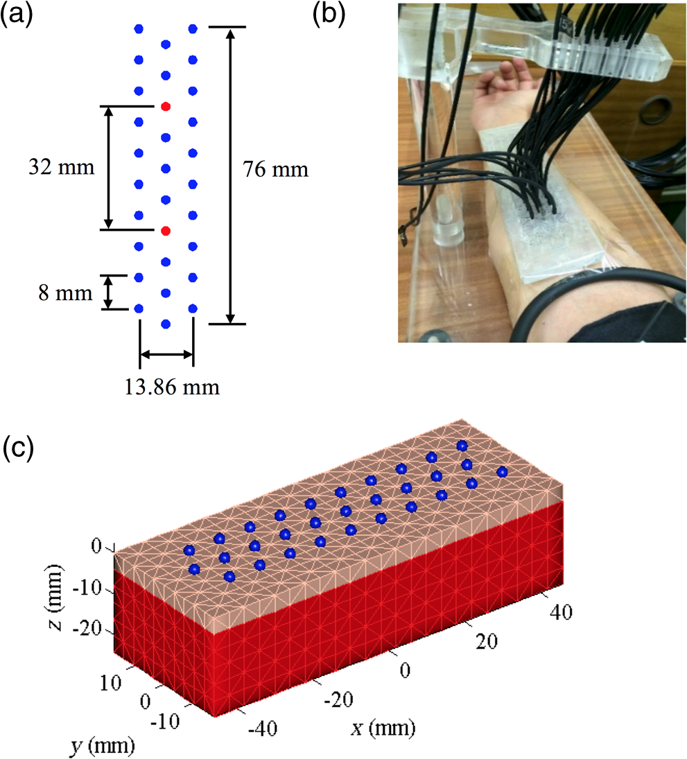

2.3.

Near-Infrared Spectroscopy

NIRS employs the modified Beer–Lambert law (MBLL)

Eq. (1)

OD = - \log \frac{I}{I_{0}} = ϵ CLB + G

to convert from changes in absorption to changes of de/oxyhemoglobin.⁵^,²⁷ In Eq. (1) OD is the optical density and

I_{0}

and

I

are incident and detected light intensities, respectively.

ϵ

represents the extinction coefficient of the tissue, and

C

is the concentration of the chromophore.

L

denotes the mean path length of detected photons.

B

is the path length factor, which accounts for the compensation of the increase of path lengths at various wavelengths caused by the scattering phenomena.

G

is defined as a geometric factor used to compensate the objective with different geometrical shapes. Typically,

L

,

B

, and

G

are constants with monochromatic illumination in a turbid media with unchanging geometry.

A change in the concentration of the chromophore causes a change in the intensity measured. The parameters $ϵ$ and $L$ remain constant, and it is assumed that $B$ and $G$ remain constant. Under this assumption, Eq. (1) can be written as

Eq. (2)

Δ OD = {OD}_{Final} - {OD}_{Initial} = - \log \frac{I_{f}}{I_{i}} = ϵ Δ CLB,

where

Δ OD

is the change in optical density.

{OD}_{Final}

and

{OD}_{Initial}

are the detected optical density and the optical density of incident light.

I_{f}

and

I_{i}

are the measured intensities before and after the change in concentration;

Δ C

is the change in concentration. In Eq. (2),

B

is often referred to as the differential pathlength factor²⁸ (DPF). DPF was determined experimentally for a number of tissues including forearm, calf, adult, and infant head.²⁹ Changes in detected light are dominated mainly by oxygenated (

{HbO}_{2}

) and deoxygenated hemoglobin (HbR) such that

Eq. (3)

{Δ OD}^{λ} = (ϵ_{{HbO}_{2}}^{λ} Δ [{HbO}_{2}] + ϵ_{HbR}^{λ} Δ [HbR]) B^{λ} L,

where

ϵ_{{HbO}_{2}}^{λ}

,

ϵ_{HbR}^{λ}

,

B^{λ}

are the extinction coefficients for oxyhemoglobin and deoxyhemoglobin and DPF at a given wavelength. By measuring the change in intensity at two wavelengths, it is possible to determine the concentration changes in

{HbO}_{2}

and HbR

Eq. (4)

Δ [HbR] = \frac{ϵ_{{HbO}_{2}}^{λ 2} \frac{{Δ OD}^{λ 1}}{B^{λ 1}} - ϵ_{{HbO}_{2}}^{λ 1} \frac{{Δ OD}^{λ 2}}{B^{λ 2}}}{(ϵ_{HbR}^{λ 1} ϵ_{{HbO}_{2}}^{λ 2} - ϵ_{HbR}^{λ 2} ε_{{HbO}_{2}}^{λ 1}) L}, Δ [{HbO}_{2}] = \frac{ϵ_{HbR}^{λ 1} \frac{{Δ OD}^{λ 2}}{B^{λ 2}} - ϵ_{HbR}^{λ 2} \frac{{Δ OD}^{λ 1}}{B^{λ 1}}}{(ϵ_{HbR}^{λ 1} ϵ_{{HbO}_{2}}^{λ 2} - ϵ_{HbR}^{λ 2} ϵ_{{HbO}_{2}}^{λ 1}) L} .

Typical source-detector separations in NIRS studies in reflectance mode are in the range 20 to 50 mm. NIRS measurements taken with the DYNOT equipment for separations larger than 45 mm were noisy (

CV > 5 %

), therefore this study was limited to a source-detector separation of

L = 32 mm

obtained by selecting the central fibers indicated with red circles in Fig. 1(a). Although DPF depends on inter-optode spacing and wavelength, experiments carried out in the forearm suggest that this parameter becomes constant for distances larger than 25 mm.²⁹^–³¹ For this study,

DPF = 4.0

was used for the calculation of concentration changes.

2.4.

Diffuse Optical Tomography

Photon transport in tissue was modeled using the diffusion approximation of the radiative transport equation.³²^,³³ This is a more accurate description of photon transport than the MBLL because it takes into account the random scattering of light produced by tissue. Consider the medium $Ω \subset R^{3}$ with boundary $\partial Ω$ , the diffusion equation in the steady-state domain is

Eq. (5)

- \nabla D (r) \nabla ϕ_{i} (r) + μ_{a} (r) ϕ_{i} = q_{i} (r), r \in Ω,

where

ϕ_{i} (r)

is the spatially varying photon fluence at

r

due to source

q_{i}

,

μ_{a}

is the absorption coefficient,

D = {[3 (μ_{a} + μ_{s}^{'})]}^{- 1}

is the diffusion coefficient, and

μ_{s}^{'}

is the reduced scattering coefficient. The source term represents an isotropic point source

q_{i} (r) = δ (r - r_{i})

located at a depth of one scattering length inside the medium (

d = 1 / μ_{s}^{'}

). The boundary condition is usually of Robin type³⁴

Eq. (6)

D (ξ) \frac{\partial ϕ_{i} (ξ)}{\partial n} + \frac{1}{2 A} ϕ_{i} (ξ) = 0, ξ \in \partial Ω,

where the term

A

accounts for the refractive index boundary mismatch at the interface. The quantity measured by a detector located at

ξ_{j} \in \partial Ω

, given the point source

q_{i} (r)

, is the outward flux

Γ_{i} (ξ_{j})

, and it is calculated from Fick’s law

Eq. (7)

Γ_{i} (ξ_{j}) = - D (ξ_{j}) \vec{n} (ξ_{j}) \cdot \nabla ϕ_{i} (ξ_{j}), ξ_{j} \in \partial Ω,

where

\vec{n} (ξ_{j})

denotes the direction of the normal vector to the boundary at the detector location

ξ_{j}

. Equations (5)–(7) constitute the forward problem in DOT, which can also be represented by a scalar operator mapping³⁵ between the space of optical parameters of interest,

μ_{a}

in this case, and the space of measurements as

Eq. (8)

y_{i, j} = Γ_{i} (ξ_{j}) = P_{i, j} [μ_{a} (r)], r \in Ω,

where

y_{i, j}

is the output of the

j

’th detector given the source

i

.

2.4.1.

Image reconstruction

3-D volumetric reconstruction of the absorption coefficient was carried out using a modified version of the normalized difference approach proposed by Pei et al.³⁶ At each sampling time $t_{k}$ , the 3-D absorption coefficient map $μ_{a} (r, t_{k}) = μ_{a_{ref}} (r) + Δ μ_{a} (r, t_{k})$ , discretized over the 3-D mesh, is determined by minimizing, using a nonlinear conjugated-gradient algorithm,³⁷ the following cost function³⁸

Eq. (9)

F = \sum_{r_{l \in Ω}} \sum_{i = 1}^{N_{s}} \sum_{j = 1}^{N_{d, i}} {\frac{\frac{y_{i, j} (t_{k})}{y_{i, j}^{0}} {\hat{P}}_{i, j} [μ_{a_{ref}} (r_{l})] - {\hat{P}}_{i, j} [μ_{a} (r_{l}, t_{k})]}{\frac{y_{i, j} (t_{k})}{y_{i, j}^{0}} \hat{P} [μ_{a_{ref}} (r_{l})]}}^{2} .

The first summation in the right side of Eq. (9) is over the volume elements of the 3-D mesh. In Eq. (9),

N_{s}

is the total number of sources,

N_{d, i}

is the number of detectors for the

i

’th source,

y_{i, j} (t_{k})

is the flux measured by the

j

’th optode given the source

i

at time

t_{k}

,

y_{i, j}^{0}

is a reference state defined as the mean of the baseline measurements, and

{\hat{P}}_{i, j} [μ_{a_{ref}} (r)]

and

{\hat{P}}_{i, j} [μ_{a} (r, t_{k})]

are the model predicted measurements for the reference and estimated absorption coefficient at time

t_{k}

. Essentially, for each time sample, the initial guess in the optimization process is the reference state

μ_{a_{ref}} (r)

. The conjugate gradient descent algorithm is applied iteratively for

n

steps to compute the estimate

μ_{a} (r, t_{k})

. Note that the optimized image from a previous time sample can be used also as the initial guess. However, in this paper, concentration calculations were carried out independently of previous or subsequent samples.

2.4.2.

Calculation of hemoglobin concentration

The absorption coefficient is related to the extinction coefficient and concentration as $μ_{a} = ε C$ . Assuming that the primary source of absorption changes is a combination of hemoglobin chromophores

Eq. (10)

Δ μ_{a} = ϵ_{{HbO}_{2}}^{λ} Δ [{HbO}_{2}] + ϵ_{HbR}^{λ} Δ [HbR],

where

ϵ_{{HbO}_{2}}^{λ}

and

ϵ_{HbR}^{λ}

are the extinction coefficients for oxyhemoglobin and deoxyhemoglobin at a given wavelength. Reconstruction of absorption changes at two different wavelengths provides two independent equations, which can be solved simultaneously to calculate deoxyhemoglobin and oxyhemoglobin concentration changes as

Eq. (11)

Δ [HbR] = \frac{ϵ_{{HbO}_{2}}^{λ 1} Δ μ_{a}^{λ 2} - ϵ_{{HbO}_{2}}^{λ 2} Δ μ_{a}^{λ 1}}{ϵ_{{HbO}_{2}}^{λ 1} ϵ_{HbR}^{λ 2} - ϵ_{{HbO}_{2}}^{λ 2} ϵ_{HbR}^{λ 1}} Δ [{HbO}_{2}] = \frac{ϵ_{HbR}^{λ 2} Δ μ_{a}^{λ 1} - ϵ_{HbR}^{λ 1} Δ μ_{a}^{λ 2} .}{ϵ_{{HbO}_{2}}^{λ 1} ϵ_{HbR}^{λ 2} - ϵ_{{HbO}_{2}}^{λ 2} ϵ_{HbR}^{λ 1}}

2.4.3.

Finite element modeling

A simplified finite element model of the skin and muscle tissue was used to implement the DOT reconstruction algorithms. The tissue was modeled as a rectangular cuboid with two layers [Fig. 1(c)] with dimensions $92 mm \times 35 mm \times 24 mm$ ( $length \times width \times depth$ ). A tetrahedral mesh with 6900 elements and 1848 nodes [Fig. 1(c)] was generated for this domain. Each layer was assigned realistic optical parameters within the range of clinically normal tissue: $μ_{a} = 0.01 {mm}^{- 1}$ and $μ_{s}^{'} = 1.00 {mm}^{- 1}$ for skin³⁹ and $μ_{a} = 0.02 {mm}^{- 1}$ and $μ_{s}^{'} = 0.50 {mm}^{- 1}$ for muscle.⁴⁰

A simulation study was carried out to calculate the photon measurement density functions for different source-detector configurations. PDMFs characterize the regions of the tissue that contribute to the measurement signal and can be used to determine a suitable combination of measurements to reconstruct optical properties of tissue within a region of interest (ROI).

It is well known that the sensitivity in the reflectance mode is higher at the surface and diminishes as function of the depth.⁴¹^,⁴² The study confirmed that for the chosen optode arrangement, depths larger than $\sim 12 mm$ contributed less than 5% to the sensitivity function. As a result, the ROI used in the analysis was a rectangular cuboid with dimensions $80 mm \times 20 mm \times 12 mm$ ( $length \times width \times depth$ ) as shown in Fig. 2.

Fig. 2

The ROI is indicated with the volume in green. The location of the optodes in relation to the ROI is indicated with the blue circles. The dimensions of the ROI are $80 mm \times 20 mm \times 12 mm$ ( $length \times width \times depth$ ). The ROI is located directly under the array of 30 optodes.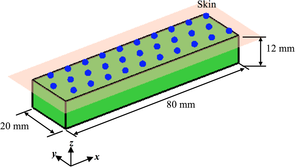

Yu et al.⁴³ showed through experiments and simulation studies that for source–detector separations larger than 1 cm, the hyperemic response is mainly influenced by the autoregulation of muscle tissue, while smaller separations are primarily affected by subcutaneous tissue layer. For this reason, first- and second-nearest neighbor source–detector pairs were not used in the reconstruction.

3-D maps of absorption changes were obtained by minimizing the cost function in Eq. (9). To minimize the occurrence of artifacts, a two-step sign constraint algorithm was used during the reconstruction process.⁴⁴ Positivity/negativity constraints were imposed after each iteration in separate reconstructions, and then the final absorption value was calculated as the sum of the two partial solutions. Positivity/negativity constraints force the algorithm to seek only positive/ negative changes in order to minimize the cost function given in Eq. (9). In each case, convergence was usually achieved after 5 to 10 iterations. Pei et al.⁴⁴ demonstrated theoretically and experimentally that by using sign constraints, the quality and specificity of the recovered images improved significantly.

Finally, Eq. (11) was used to compute ${HbO}_{2}$ , HbR, and HbT ( ${HbO}_{2} + HbR$ ). Near-infrared parameters of postocclusive reactive hyperemia (PORH) were calculated on a nodal basis and then averaged on the ROI.

2.5.

Study Protocol

The weight, height, and age for each subject were recorded. The baseline characteristics of the subjects are summarized in Table 1. Microvascular function during forearm PORH was assessed on two different occasions 1 to 2 weeks apart. In order to assess “real-world” performance, subjects were not asked to fast or abstain from exercise, and the time of day of assessment was not standardized. Subjects were requested to sit comfortably on a chair and to locate the right arm on a platform such that the dorsal-ventral axis of the elbow was held parallel to the surface of the platform [Fig. 1(b)]. The hand was placed such that the palm was facing upward. A manual pneumatic blood pressure cuff was placed above the elbow, and the tomographic probe was placed on the ventral side of the forearm on the brachioradialis muscle and attached with tape [Fig. 1(a)].

The test consisted of 3 min baseline, followed by 5 min of arterial occlusion (induced by inflating the cuff to 180 mmHg). After 5 min, the cuff was rapidly deflated and the response measured for a further 5 min (13 min total measurement time). Light attenuation changes were recorded at the four wavelengths, but only the data at 760 and 830 nm were used for processing. Hemodynamics changes were calculated using NIRS and DOT techniques. The former uses the MBLL to convert absorption changes into de/oxyhemoglobin⁵^,²⁷ [Eq. (4)], while the latter is based in the diffusion process of light [Eqs. (5) and (6)].³⁵

The parameters measured during and after the arterial occlusion test are (Fig. 3):

(i) ${mVO}_{2}$ ( $ml O_{2} / \min / 100 g$ ), muscle oxygen consumption: calculated from the gradient of the ${HbO}_{2}$ at the beginning of the arterial occlusion and converted into ml $O_{2} / \min / 100 g$ .¹⁰
(ii) $1 / 2$ ${THbO}_{2}$ (s), $1 / 2$ time of recovery of ${HbO}_{2}$ : time needed for half recovery of ${HbO}_{2}$ from maximum deoxygenation at the end of the occlusion period to maximum reoxygenation during reactive hyperemia.
(iii) ${THbO}_{2}$ (s), time to maximal ${HbO}_{2}$ : time interval after cuff release until maximum ${HbO}_{2}$ value is reached.
(iv) ${MaxHbO}_{2}$ ( $μ M$ ), maximal amplitude of ${HbO}_{2}$ : maximal hyperemic response reached by ${HbO}_{2}$ .
(v) MaxHbT ( $μ M$ ), maximal amplitude of HbT: maximal hyperemic response of HbT.
(vi) THbT (s), time to maximal HbT: time to peak value of HbT after cuff release.
(vii) Increase rate to maximal ${HbO}_{2}$ ( $μ M / s$ ), reoxygenation rate of ${HbO}_{2}$ : calculated by dividing Max ${HbO}_{2}$ by the time to maximal ${HbO}_{2}$ .
(viii) Increase rate to maximal HbT ( $μ M / s$ ), reoxygenation rate of HbT: calculated by dividing Max HbT by the time and maximal HbT.
(ix) AUC ${HbO}_{2}$ (a.u.), area under the curve of ${HbO}_{2}$ after cuff release.
(x) AUC HbR (a.u.), postocclusion area under the curve of HbT.
(xi) AUC HbT (a.u.), area under the curve of HbT after cuff release.

Fig. 3

Typical hemodynamic response before, during, and after 5 min brachial arterial occlusion measured by NIRS. Some characteristic parameters are indicated: oxygen consumption ( ${mVO}_{2}$ ), maximal amplitude of ${HbO}_{2}$ (Max. ${HbO}_{2}$ ), time to maximal of ${HbO}_{2}$ ( ${THbO}_{2}$ ), and area under the curve of ${HbO}_{2}$ (AUC).

The reproducibility was assessed using the intraclass correlation coefficient (ICC) and the standard error of measurement (SEM)⁴⁵ based on NIRS parameters measured on two separate occasions. ICC provides the degree to which individuals maintain their rank order across repeated tests, and SEM is a measure of absolute repeatability. To interpret repeatability based on ICC values, the following guidelines were considered:⁴⁶ $ICC \geq 0.8$ indicates “excellent,” $0.6 \leq ICC < 0.8$ is defined as “good,” $0.4 \leq ICC < 0.6$ indicates “moderate,” $0.2 \leq ICC < 0.4$ indicates “fair,” and $ICC < 0.2$ is defined as “poor.” On the other hand, SEM is expressed as a percentage and the ideal value is zero. In general, the smaller the SEM, the smaller the variability between individual repeated measurements. ICC was calculated for near-infrared parameters derived using DOT and NIRS, and this is denoted by ${ICC}_{DOT}$ and ${ICC}_{NIRS}$ , respectively (similarly for SEM: ${SEM}_{DOT}$ and ${SEM}_{NIRS}$ ).

3. Results

3.1.

Microvascular Function Reproducibility

Table 2 lists the mean and standard deviation of near-infrared parameters, calculated using DOT, during and after the arterial occlusion test, together with ICC and SEM repeatability measures. Similarly, Table 3 displays mean and standard deviation of near-infrared parameters measured using NIRS. Mean values in both tables are very similar; however, the standard deviation for near-infrared parameters derived using DOT is smaller in most cases. More importantly, the ${ICC}_{DOT}$ is higher in all but one case, and the repeatability is extremely high ( $\sim 1$ ) for ${mVO}_{2}$ , ${THbO}_{2}$ , Max. ${HbO}_{2}$ , and THbT. In comparison, only one parameter ( ${mVO}_{2}$ ) measured with NIRS reached the “excellent” ICC category. The least repeatable parameter is AUC HbR, and this is consistent in the two measuring approaches.

Table 2

Intrasubject reproducibility of PORH parameters obtained using DOT.

Parameter	Test 1	Test 2	ICC	SEM
${mVO}_{2}$	$0.07 \pm 0.02$	$0.07 \pm 0.03$	0.99	3.90
$1 / 2 {THbO}_{2}$	$14.34 \pm 2.33$	$15.17 \pm 1.82$	0.72	7.50
${THbO}_{2}$	$36.50 \pm 10.44$	$36.81 \pm 7.70$	0.94	6.09
${MaxHbO}_{2}$	$19.99 \pm 6.06$	$20.01 \pm 7.31$	0.99	2.85
MaxHbT	$19.21 \pm 5.24$	$20.09 \pm 6.92$	0.69	17.31
THbT	$21.63 \pm 13.35$	$21.71 \pm 7.98$	0.99	5.98
Inc. rate to max ${HbO}_{2}$	$1.53 \pm 0.51$	$1.46 \pm 0.55$	0.70	19.60
Inc. rate to max HbT	$0.72 \pm 0.39$	$0.62 \pm 0.47$	0.51	45.16
AUC ${HbO}_{2}$	$1461.79 \pm 572.51$	$1625.32 \pm 900.88$	0.54	32.22
AUC HbR	$708.47 \pm 586.48$	$611.91 \pm 551.93$	0.63	52.11
AUC HbT	$1313.68 \pm 963.06$	$1741.28 \pm 775.31$	0.22	45.11

Table 3

Intrasubject reproducibility of PORH parameters obtained using NIRS spectroscopy.

Parameter	Test 1	Test 2	ICC	SEM
${mVO}_{2}$	$0.08 \pm 0.06$	$0.08 \pm 0.04$	0.97	10.98
$1 / 2 {THbO}_{2}$	$16.57 \pm 11.18$	$15.64 \pm 3.29$	0.64	26.82
${THbO}_{2}$	$45.90 \pm 18.63$	$47.79 \pm 17.56$	0.77	18.55
${MaxHbO}_{2}$	$16.56 \pm 4.66$	$15.85 \pm 4.46$	0.67	16.29
MaxHbT	$17.72 \pm 6.08$	$16.01 \pm 4.42$	0.37	24.70
THbT	$19.90 \pm 2.88$	$20.69 \pm 6.38$	0.71	12.25
Inc. rate to max ${HbO}_{2}$	$1.06 \pm 0.52$	$0.85 \pm 0.38$	0.21	41.94
Inc. rate to max HbT	$0.73 \pm 0.40$	$0.60 \pm 0.45$	0.40	50.17
AUC ${HbO}_{2}$	$1053.21 \pm 740.53$	$1131.97 \pm 838.85$	0.78	33.89
AUC HbR	$810.67 \pm 657.29$	$1016.41 \pm 840.48$	0.45	61.01
AUC HbT	$1385.63 \pm 929.66$	$1897.82 \pm 836.57$	0.19	48.47

SEM calculated for tomographic imaging showed consistently smaller values across all parameters. This suggests that region-wise averaged measurements provide more robust and repeatable measurements than point-wise measurements, as typically measured in NIRS.

4. Discussion

Our results are in agreement with similar studies using NIRS;²⁰^,⁴⁷ however, the main finding is that tomographic imaging provides more robust and repeatable results. Figure 4 shows the mean and SEM of de/oxyhemoglobin and total hemoglobin across all subjects computed using NIRS and DOT. NIRS calculations are noisier than DOT reconstructions, despite using the same filtering techniques in both methods. One reason might be that single-channel measurements are more susceptible to systematic errors, such as position-dependent differences in muscle oxygenation or probe localization and interobserver reproducibility. On the other hand, DOT samples a larger tissue volume. Averaging over a large number of voxels also smooths the response. Furthermore, the image reconstruction method for DOT implements regularization that further improves the SNR.⁸

Fig. 4

Average (solid lines) and standard deviation (vertical bars) of ${HbO}_{2}$ , HbR, and HbT responses across all subjects in the first experiment obtained using (a) NIRS spectroscopy and (b) DOT.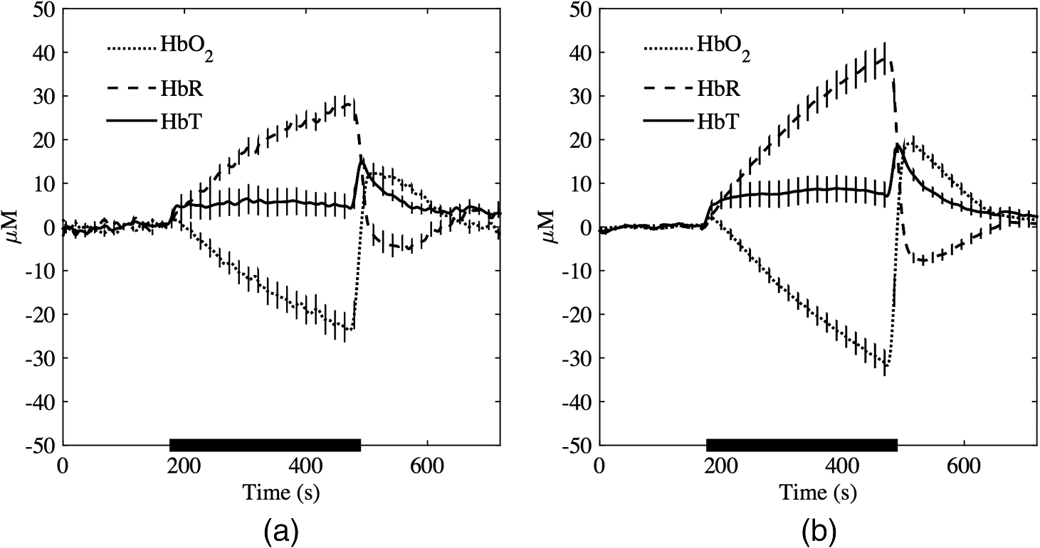

Figure 5(a) shows the volume averaged ${HbO}_{2}$ , HbR, and HbT for a representative subject while Fig. 5(b) shows a tomographic reconstruction for ${HbO}_{2}$ at its maximum value ( $t = 516 s$ ). The heterogeneity of tissue is evident, and this has been reported in similar studies involving two-dimensional images of venous occlusion tests.⁴⁸ Furthermore, spatial dependence of the hemodynamic responses in the forearm has also been reported in nerve stimulation studies⁴⁹ and in exercising hand in the reflectance⁵⁰ and transmittance⁵¹ modes. This variability that occurs in all three spatial directions may contribute to diminished repeatability if the probe location is not consistent across examinations.

Fig. 5

(a) Typical hemodynamic responses of oxygenated ( ${HbO}_{2}$ ), de-oxygenated (HbR) and total hemoglobin (HbT) and (b) ${HbO}_{2}$ $(x, y, z, t)$ at $t = 516 s$ , i.e., the time average ${HbO}_{2}$ reaches maximum.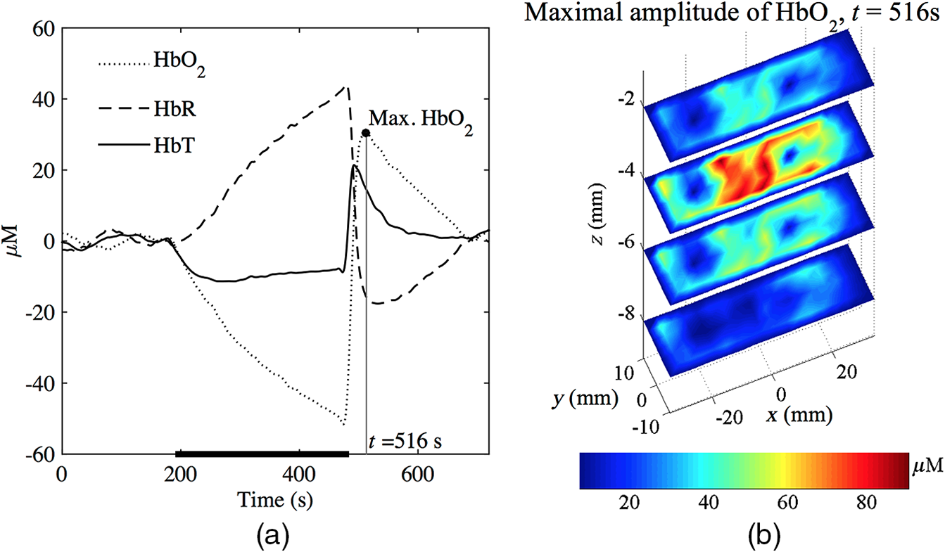

NIRS and DOT calculations have clear methodological differences, both prone to systematic errors. For NIRS, the key parameter is the DPF, which corrects for the effect of scattering in tissue and therefore is wavelength and tissue dependent. This variable has been the subject of several investigations, and there is an agreement on its main characteristics at population levels.²⁹^–³¹^,⁵² However, in most of the cases, DPF is not calculated as part of the arterial/venous occlusion protocol, and calculations are based on data and tables available in the literature.

The techniques used in DOT are more complex and also susceptible to systematic errors such as parameterization of optical parameters, initial guess, or reconstruction convergence criteria. In this study, a differential approach was followed, which has demonstrated to be insensitive to boundary effects and the medium’s initial guess.³⁶ On the other hand, the major disadvantage is that it is not possible to determine the absolute distribution of optical parameters, but only the change of absorption or diffusion from a given baseline.

In general, our results show time-based parameters have excellent repeatability. These parameters have shown great promise in distinguishing between healthy volunteers and patients with PAD and diabetes.¹⁶^,¹⁷ For these patient groups, the reactive hyperemic response showed delayed times of recovery. Parameters derived from ${HbO}_{2}$ are also the most repeatable, and this has been observed by different groups.¹⁶^,²⁰^,²¹

4.1.

Regions of Hemodynamic Consistence

The availability of 3-D maps allows the selection of more specific areas of interest. Selection techniques, either manual or automatic, are available and have been shown to enhance the response by improving the signal-to-noise ratio. Wang⁵³ used a binarized segmentation technique to select the regions with the dominant response, while in another study by Cuccia et al.,⁵⁴ regions with large vessels were avoided to focus on regions containing only microvasculature. Recently, Khalil et al.⁵⁵ employed correlation analysis to define regions of temporal consistency that correlate significantly with the averaged HbT. Their results showed some differences in the evolution of HbT between a healthy volunteer and a patient with PAD, which were not evident from the average signals alone.

The best selection strategy is likely to be disease-dependent, and for this reason, we did not attempt to develop one based only on healthy volunteer subjects. However, to illustrate the potential advantages of DOT compared with NIRS, we carried out the following simple analysis:

Step 1. Compute the average total hemoglobin time series over the ROI, denoted by ${HbT}_{ROI} (t)$ , and determine the time point satisfying
${HbT}_{ROI} (t_{\max}) = \max [{HbT}_{ROI} (t)] .$
This point is located at $t_{\max} = 467 s$ [Fig. 6(a)].
Step 2. Determine the node $(x_{M}, y_{M}, z_{M})$ satisfying
$HbT (x_{M}, y_{M}, z_{M}, t) = \max [HbT (x, y, z, t)]$
for $t = 467 s$ [Fig. 6(b)].
Step 3. For each node $(x_{i}, y_{i}, z_{i})$ within the ROI, compute the cross-correlation between $HbT (x_{M}, y_{M}, z_{M}, t) = {HbT}_{\max} (t)$ and $HbT (x_{i}, y_{i}, z_{i}, t) = {HbT}_{i} (t)$ using
Eq. (12)
$ρ (x_{i}, y_{i}, z_{i}) = \frac{\sum_{k = 1}^{N} [{HbT}_{i} (k) - {\bar{HbT}}_{i}] [{HbT}_{\max} (k) - {\bar{HbT}}_{\max}]}{\sum_{k = 1}^{N} \sqrt{{[{HbT}_{i} (k) - {\bar{HbT}}_{i}]}^{2}} \sum_{t = 0}^{N - 1} \sqrt{{[{HbT}_{ref} (k) - {\bar{HbT}}_{\max}]}^{2}}},$
where $N$ is the total number of samples and the bar over each variable denotes the time average over the duration of the experiment. The analysis was done on the entire experiment to illustrate the different dynamic signatures that can be obtained when different reference signals are used. Note also that ${HbT}_{\max} (t)$ is not necessarily the time series with the highest HbT across the experiment.

The resulting 3-D correlation map $ρ (x, y, z)$ , shown in Fig. 6(c), indicates very strong correlation ( $ρ_{i} > 0.9$ ) with the reactive hyperemic response ${HbT}_{\max} (t)$ for nodes located at a depth $> \sim 2 mm$ , which largely correspond to muscle tissue.

Fig. 6

(a) Total hemoglobin curve (HbT) for a healthy subject; the point at maximal HbT ( $t = 467 s$ ) is marked with a point. (b) 3-D map of $HbT (x, y, z)$ at the time of maximal HbT. The node with maximum contribution to the HbT response, $HbT (x_{M}, y_{M}, z_{M})$ , is indicated by the arrow and its time response is denoted with ${HbT}_{\max} (t)$ . (c) 3-D map of correlation coefficients $ρ (x, y, z)$ computed between ${HbT}_{i} (t)$ at each node location ( $x_{i}$ , $y_{i}$ , $z_{i}$ ) and ${HbT}_{\max} (t)$ . (d) 3-D map of correlation coefficients $ρ (x, y, z)$ computed between ${HbT}_{i} (t)$ at each node location ( $x_{i}$ , $y_{i}$ , $z_{i}$ ) and ${HbT}_{mean} (t)$ .

In contrast, the correlation coefficients for nodes located in the superficial layer (skin) are very low ( $ρ_{i} \leq 0.4$ ). A different correlation map was computed using as a reference the averaged HbT signal over the ROI, denoted ${HbT}_{ROI} (t)$ .

The corresponding 3-D correlation map, shown in Fig. 6(d), also exhibits strong correlation for nodes ( $ρ_{i} > 0.9$ ) located bellow the skin layer. The correlation maps can be used to define tissue compartments with similar hemodynamic profiles. For example, regions of hemodynamic consistency (RHC) can be defined based on the correlation maps shown in Fig. 6(c) and 6(d) by selecting all nodes with correlation coefficient $ρ \geq 0.9$ .

The resulting RHCs are shown in Fig. 7(a); the red and green volumes indicate the regions with high correlation ( $ρ \geq 0.9$ ) with the ${HbT}_{mean}$ and ${HbT}_{\max} (t)$ , respectively. The blue volume represents the intersection between the two RHC. The average HbT time series for each RHC are shown in Fig. 7(b) together with the averaged HbT over the entire ROI $[{HbT}_{ROI} (t)]$ .

Fig. 7

(a) Compartments defined by the two RHC: the A and B volumes indicate the regions with high correlation ( $ρ \geq 0.9$ ) with the ${HbT}_{mean} (t)$ and ${HbT}_{\max} (t)$ , respectively. The AB represent the intersection between the the A and B regions. The boundaries of the ROI are denoted with the black box. (b) Total hemoglobin averaged over the entire ROI $[{HbT}_{mean} (t)]$ is indicated with the solid line. The dashed and dotted lines denote the average HbT response of all the nodes with high correlation ( $ρ \geq 0.9$ ) with ${HbT}_{mean} (t)$ and ${HbT}_{\max} (t)$ , respectively.

Interestingly, while the three signals are different before the end of the occlusion period, after the cuff is released only the region correlated to ${HbT}_{\max} (t)$ is still distinct compared with the average signal over the entire ROI. This tissue “compartment” identified by our analysis [Fig. 7(a)] appears to exhibit extensive reactive hyperemia both in terms of significantly increased blood flow relative to the baseline as well as duration of hyperemia.

The DOT-estimated MaxHbT and ${MaxHbO}_{2}$ also have good reproducibility ( $ICC = 0.69$ and $ICC = 0.99$ , respectively), suggesting that an RHC identified based on ${HbT}_{\max} (t)$ could be a good candidate to focus on in future studies that aim to distinguish between healthy volunteers and patients with vascular disorder.

In contrast, the relatively poor reproducibility of MaxHbT measured using NIRS ( $ICC = 0.37$ ), which clearly limits its diagnostic potential, highlights the challenges posed by the spatial and temporal heterogeneity of tissue oxygenation and hemodynamics when assessing endothelial function.

To further illustrate the advantage of using DOT to resolve the spatiotemporal properties of the hemodynamic response, we created a short movie (Fig. 8) showing the reconstructed HbT changes in different slice planes along the $x$ axis.

Fig. 8

(a) Dynamical changes of ${HbO}_{2}$ (dotted line), HbR (dashed line), and HbT (solid line) for a healthy volunteer. (Video 1, top panel) The vertical line indicates the specific time point where a tomographic map is displayed in the lower panel. (b) Visualization of volumetric changes of HbT (video 1, bottom panel) using $y - z$ slice planes located at $x = - 30$ , $- 15$ , 0, 15, and 30 mm. (Video 1, MPEG-4, 941 KB) [URL: http://dx.doi.org/10.1117/1.JBO.21.6.066012.1].

5. Conclusions

This study shows that DOT achieves excellent reproducibility of key PORH parameters. These parameters include muscle oxygen consumption ( ${mVO}_{2}$ ), time to maximal ${HbO}_{2}$ ( ${THbO}_{2}$ ), maximal ${HbO}_{2}$ ( ${MaxHbO}_{2}$ ), and time to maximal HbT (THbT). Although a direct comparison of these parameters may be enough to distinguish between healthy volunteers and patients with vascular disease, our analysis suggests that obtaining reliable signatures of vascular disease may require first the identification of an appropriate RHC. This is only possible if a full volumetric reconstruction of hemodynamics, as that provided by DOT, is available for the particular ROI. The choice of an appropriate RHC is beyond the scope of this study, and it is the subject of future research.

The availability of volumetric hemodynamic parameters clearly offers more opportunities for the analysis and characterization of PORH and warrants further efforts to evaluate DOT’s potential to measure endothelial function in a clinical environment.

Despite the increased complexity of the instrumentation and reconstruction algorithms used to implement DOT, there are many examples of inexpensive portable and wearable DOT instruments.⁵⁶ The availability of freely available software such as NIRFAST⁵⁷ and TOAST⁵⁸ also encourages the development of DOT-based technology. The use of reduced-order models¹⁴ to speed up the reconstruction process makes it now possible to perform analyses in real-time using mobile devices with modest computational resources.

Overall, the inherent advantages of DOT compared with other imaging modalities, combined with the availability of algorithms and portability of the instrumentation, makes DOT an ideal method for routinely and noninvasively assessing the cardiovascular function, inside and outside the hospital.

Acknowledgments

The authors gratefully acknowledge that this work was supported by the University of Sheffield as part of the “Engineering for Life” 2022 Futures Project and by EPSRC grants EP/H00453X/1 (S.A.B. and D.C.) and GR/T01006/01 (D.C.), by BBSRC grant BB/K010123/1 (S.A.B. and D.C.) and by an ERC Advanced Investigator Grant (S.A.B.). E.E.V.R. gratefully acknowledges the support from a grant from the Mexican National Research Council for Science and Technology (CONACYT).

References

1.

G. A. Roth et al., “Global and regional patterns in cardiovascular mortality from 1990 to 2013,” Circulation, 132 (17), 1667 –1678 (2015). http://dx.doi.org/10.1161/CIRCULATIONAHA.114.008720 JBOPFOCIRCAZ 1083-36680009-7322 Google Scholar

2.

Cardiovascular Disease Outcomes Strategy, 89 Department of Health, London (2013). Google Scholar

3.

D. A. Benaron et al., “Noninvasive methods for estimating in vivo oxygenation,” Clin. Pediatr., 31 (5), 258 –273 (1992). http://dx.doi.org/10.1177/000992289203100501 Google Scholar

4.

M. Ferrari, M. Muthalib and V. Quaresima, “The use of near-infrared spectroscopy in understanding skeletal muscle physiology: recent developments,” Philos. Trans. R Soc. A, 369 (1955), 4577 –4590 (2011). http://dx.doi.org/10.1098/rsta.2011.0230 Google Scholar

5.

M. Cope and D. T. Delpy, “System for long-term measurement of cerebral blood and tissue oxygenation on newborn-infants by near-infrared trans-illumination,” Med. Biol. Eng. Comput., 26 (3), 289 –294 (1988). http://dx.doi.org/10.1007/BF02447083 MBECDY 0140-0118 Google Scholar

6.

F. F. Jobsis, “Noninvasive, infrared monitoring of cerebral and myocardial oxygen sufficiency and circulatory parameters,” Science, 198 (4323), 1264 –1267 (1977). http://dx.doi.org/10.1126/science.929199 SCIEAS 0036-8075 Google Scholar

7.

D. A. Boas, A. M. Dale and M. A. Franceschini, “Diffuse optical imaging of brain activation: approaches to optimizing image sensitivity, resolution, and accuracy,” Neuroimage, 23 S275 –S288 (2004). http://dx.doi.org/10.1016/j.neuroimage.2004.07.011 NEIMEF 1053-8119 Google Scholar

8.

A. P. Gibson, J. C. Hebden and S. R. Arridge, “Recent advances in diffuse optical imaging,” Phys. Med. Biol., 50 (4), R1 –R43 (2005). http://dx.doi.org/10.1088/0031-9155/50/4/R01 PHMBA7 0031-9155 Google Scholar

9.

A. Villringer and B. Chance, “Non-invasive optical spectroscopy and imaging of human brain function,” Trends Neurosci., 20 (10), 435 –442 (1997). http://dx.doi.org/10.1016/S0166-2236(97)01132-6 TNSCDR 0166-2236 Google Scholar

10.

M. C. P. Van Beekvelt et al., “Performance of near-infrared spectroscopy in measuring local O 2 consumption and blood flow in skeletal muscle,” J. Appl. Physiol., 90 (2), 511 –519 (2001). Google Scholar

11.

D. A. Boas et al., “The accuracy of near infrared spectroscopy and imaging during focal changes in cerebral hemodynamics,” Neuroimage, 13 (1), 76 –90 (2001). http://dx.doi.org/10.1006/nimg.2000.0674 NEIMEF 1053-8119 Google Scholar

12.

C. Habermehl et al., “Somatosensory activation of two fingers can be discriminated with ultrahigh-density diffuse optical tomography,” NeuroImage, 59 (4), 3201 –3211 (2012). http://dx.doi.org/10.1016/j.neuroimage.2011.11.062 NEIMEF 1053-8119 Google Scholar

13.

G. Strangman, M. A. Franceschini and D. A. Boas, “Factors affecting the accuracy of near-infrared spectroscopy concentration calculations for focal changes in oxygenation parameters,” Neuroimage, 18 (4), 865 –879 (2003). http://dx.doi.org/10.1016/S1053-8119(03)00021-1 NEIMEF 1053-8119 Google Scholar

14.

E. E. Vidal-Rosas et al., “Reduced-order modeling of light transport in tissue for real-time monitoring of brain hemodynamics using diffuse optical tomography,” J. Biomed. Opt., 19 (2), 026008 (2014). http://dx.doi.org/10.1117/1.JBO.19.2.026008 JBOPFO 1083-3668 Google Scholar

15.

M. Vardi and A. Nini, “Near-infrared spectroscopy for evaluation of peripheral vascular disease. a systematic review of literature,” Eur. J. Vasc. Endovascular Surg., 35 (1), 68 –74 (2008). http://dx.doi.org/10.1016/j.ejvs.2007.07.015 Google Scholar

16.

T. Jarm et al., “Postocclusive reactive hyperemia in healthy volunteers and patients with peripheral vascular disease measured by three noninvasive methods,” Advances in Experimental Medicine and Biology, 661 –669 Springer, Boston, Massachusetts (2003). Google Scholar

17.

R. Kragelj et al., “Parameters of postocclusive reactive hyperemia measured by near infrared spectroscopy in patients with peripheral vascular disease and in healthy volunteers,” Ann. Biomed. Eng., 29 (4), 311 –320 (2001). http://dx.doi.org/10.1114/1.1359451 ABMECF 0090-6964 Google Scholar

18.

M. Gayda et al., “Muscle VO2 and forearm blood flow repeatability during venous and arterial occlusions in healthy and coronary heart disease subjects,” Clin. Hemorheol. Microcirculation, 59 (2), 177 –183 (2015). http://dx.doi.org/10.3233/CH-141836 Google Scholar

19.

R. C. Mesquita et al., “Diffuse optical characterization of an exercising patient group with peripheral artery disease,” J. Biomed. Opt., 18 (5), 057007 (2013). http://dx.doi.org/10.1117/1.JBO.18.5.057007 JBOPFO 1083-3668 Google Scholar

20.

S. Lacroix et al., “Reproducibility of near-infrared spectroscopy parameters measured during brachial artery occlusion and reactive hyperemia in healthy men,” J. Biomed. Opt., 17 (7), 077010 (2012). http://dx.doi.org/10.1117/1.JBO.17.7.077010 Google Scholar

21.

R. Kragelj, T. Jarm and D. Miklavcic, “Reproducibility of parameters of postocclusive reactive hyperemia measured by near infrared spectroscopy and transcutaneous oximetry,” Ann. Biomed. Eng., 28 (2), 168 –173 (2000). http://dx.doi.org/10.1114/1.241 INPEEYABMECF 0266-56110090-6964 Google Scholar

22.

M. A. Khalil et al., “Detection of peripheral arterial disease within the foot using vascular optical tomographic imaging: a clinical pilot study,” Eur. J. Vasc. Endovascular Surg., 49 (1), 83 –89 (2015). http://dx.doi.org/10.1016/j.ejvs.2014.10.010 Google Scholar

23.

A. Torricelli et al., “Functional brain imaging by multi-wavelength time-resolved near infrared spectroscopy,” Opto-electron. Rev., 16 (2), 131 –135 (2008). http://dx.doi.org/10.2478/s11772-008-0011-6 OELREM 1230-3402 Google Scholar

24.

T. Muehlemann, D. Haensse and M. Wolf, “Wireless miniaturized in-vivo near infrared imaging,” Opt. Express, 16 (14), 10323 –10330 (2008). http://dx.doi.org/10.1364/OE.16.010323 OPEXFF 1094-4087 Google Scholar

25.

K. J. Kek et al., “Optical imaging instrument for muscle oxygenation based on spatially resolved spectroscopy,” Opt. Express, 16 (22), 18173 –18187 (2008). http://dx.doi.org/10.1364/OE.16.018173 OPEXFF 1094-4087 Google Scholar

26.

C. H. Schmitz et al., “Dynamic studies of small animals with a four-color diffuse optical tomography imager,” Rev. Sci. Instrum., 76 (9), 094302 (2005). http://dx.doi.org/10.1063/1.2038467 RSINAK 0034-6748 Google Scholar

27.

M. Cope, The Development of a Near-Infrared Spectroscopy System and Its Application for Noninvasive Monitoring of Cerebral Blood and Tissue Oxygenation, University College London, London (1991). Google Scholar

28.

D. T. Delpy et al., “Estimation of optical pathlength through tissue from direct time of flight measurement,” Phys. Med. Biol., 33 (12), 1433 –1442 (1988). http://dx.doi.org/10.1088/0031-9155/33/12/008 PHMBA7 0031-9155 Google Scholar

29.

P. Van der Zee et al., “Experimentally measured optical pathlengths for the adult head, calf and forearm and the head of the newborn infant as a function of inter optode spacing,” Adv. Exp. Med. Biol., 316 143 –153 (1992). http://dx.doi.org/10.1007/978-1-4615-3404-4 AEMBAP 0065-2598 Google Scholar

30.

A. Duncan et al., “Optical pathlength measurements on adult head, calf and forearm and the head of the newborn-infant using phase-resolved optical spectroscopy,” Phys. Med. Biol., 40 (2), 295 –304 (1995). http://dx.doi.org/10.1088/0031-9155/40/2/007 PHMBA7 0031-9155 Google Scholar

31.

M. Ferrari et al., “Time-resolved spectroscopy of the human forearm,” J. Photochem. Photobiol. B, 16 (2), 141 –153 (1992). http://dx.doi.org/10.1016/1011-1344(92)80005-G JPPBEG 1011-1344 Google Scholar

32.

S. R. Arridge, “Methods in diffuse optical imaging,” Philos. Trans. R. Soc. A, 369 (1955), 4558 –4576 (2011). http://dx.doi.org/10.1098/rsta.2011.0311 PTRMAD 1364-503X Google Scholar

33.

M. S. Patterson, B. Chance and B. C. Wilson, “Time resolved reflectance and transmittance for the noninvasive measurement of tissue optical-properties,” Appl. Opt., 28 (12), 2331 –2336 (1989). http://dx.doi.org/10.1364/AO.28.002331 APOPAI 0003-6935 Google Scholar

34.

M. Schweiger et al., “The finite element method for the propagation of light in scattering media: boundary and source conditions,” Med. Phys., 22 (11), 1779 –1792 (1995). http://dx.doi.org/10.1118/1.597634 MPHYA6 0094-2405 Google Scholar

35.

S. R. Arridge, “Optical tomography in medical imaging,” Inverse Prob., 15 (2), R41 –R93 (1999). http://dx.doi.org/10.1088/0266-5611/15/2/022 Google Scholar

36.

Y. L. Pei, H. L. Graber and R. L. Barbour, “Influence of systematic errors in reference states on image quality and on stability of derived information for dc optical imaging,” Appl. Opt., 40 (31), 5755 –5769 (2001). http://dx.doi.org/10.1364/AO.40.005755 JBOPFOAPOPAI 1083-36680003-6935 Google Scholar

37.

J. Nocedal and S. Wright, Numerical Optimization, 2nd Ed.Springer, New York (2006). Google Scholar

38.

A. Y. Bluestone et al., “Three-dimensional optical tomographic brain imaging in small animals, part 1: hypercapnia,” J. Biomed. Opt., 9 (5), 1046 –1062 (2004). http://dx.doi.org/10.1117/1.1784471 Google Scholar

39.

T. Lister, P. A. Wright and P. H. Chappell, “Optical properties of human skin,” J. Biomed. Opt., 17 (9), 090901 (2012). http://dx.doi.org/10.1117/1.JBO.17.9.090901 Google Scholar

40.

S. L. Jacques, “Optical properties of biological tissues: a review,” Phys. Med. Biol., 58 (11), R37 –R61 (2013). http://dx.doi.org/10.1088/0031-9155/58/11/R37 PHMBA7 0031-9155 Google Scholar

41.

S. R. Arridge and M. Schweiger, “Photon-measurement density-functions. 2. Finite-element-method calculations,” Appl. Opt., 34 (34), 8026 –8037 (1995). http://dx.doi.org/10.1364/AO.34.008026 APOPAI 0003-6935 Google Scholar

42.

S. R. Arridge, “Photon-measurement density functions. Part I: analytical forms,” Appl. Opt., 34 (31), 7395 –7409 (1995). http://dx.doi.org/10.1364/AO.34.007395 APOPAI 0003-6935 Google Scholar

43.

G. Q. Yu et al., “Time-dependent blood flow and oxygenation in human skeletal muscles measured with noninvasive near-infrared diffuse optical spectroscopies,” J. Biomed. Opt., 10 (2), 024027 (2005). http://dx.doi.org/10.1117/1.1884603 JBOPFO 1083-3668 Google Scholar

44.

Y. L. Pei, H. L. Graber and R. L. Barbour, “Normalized-constraint algorithm for minimizing inter-parameter crosstalk in DC optical tomography,” Opt. Express, 9 (2), 97 –109 (2001). http://dx.doi.org/10.1364/OE.9.000097 OPEXFF 1094-4087 Google Scholar

45.

T. A. Baumgartner, “Statistical tools in evaluation,” Statistical Tools in Evaluation, 3rd Ed.Houghton Mifflin, London (1987). Google Scholar

46.

D. G. Altman, Practical Statistics for Medical Research, 623 Chapman & Hall, London (1999). Google Scholar

47.

M. C. P. van Beekvelt et al., “In vivo quantitative near-infrared spectroscopy in skeletal muscle during incremental isometric handgrip exercise,” Clin. Physiol. Funct. Imaging, 22 (3), 210 –217 (2002). http://dx.doi.org/10.1046/j.1475-097X.2002.00420.x Google Scholar

48.

C. Casavola et al., “Blood flow and oxygen consumption with near-infrared spectroscopy and venous occlusion: spatial maps and the effect of time and pressure of inflation,” J. Biomed. Opt., 5 (3), 269 –276 (2000). http://dx.doi.org/10.1117/1.429995 JBOPFO 1083-3668 Google Scholar

49.

D. K. Chen et al., “Spectral and spatial dependence of diffuse optical signals in response to peripheral nerve stimulation,” Biomed. Opt. Express, 1 (3), 923 –942 (2010). http://dx.doi.org/10.1364/BOE.1.000923 BOEICL 2156-7085 Google Scholar

50.

M. Maris et al., “Functional near-infrared imaging of deoxygenated hemoglobin during exercise of the finger extensor muscles using the frequency-domain technique,” Bioimaging, 2 (4), 174 –183 (1994). http://dx.doi.org/10.1002/1361-6374(199412)2:4<174::AID-BIO2>3.3.CO;2-H BOIMEL 0966-9051 Google Scholar

51.

E. M. C. Hillman et al., “Time resolved optical tomography of the human forearm,” Phys. Med. Biol., 46 (4), 1117 –1130 (2001). http://dx.doi.org/10.1088/0031-9155/46/4/315 PHMBA7 0031-9155 Google Scholar

52.

S. J. Matcher, M. Cope and D.T. Delpy, “In vivo measurements of the wavelength dependence of tissue-scattering coefficients between 760 and 900 nm measured with time-resolved spectroscopy,” Appl. Opt., 36 (1), 386 –396 (1997). http://dx.doi.org/10.1364/AO.36.000386 APOPAI 0003-6935 Google Scholar

53.

C. Y. Wang et al., “Diffuse optical multipatch technique for tissue oxygenation monitoring: clinical study in intensive care unit,” IEEE Trans. Biomed. Eng., 59 (1), 87 –94 (2012). http://dx.doi.org/10.1109/TBME.2011.2147315 IEBEAX 0018-9294 Google Scholar

54.

D. J. Cuccia et al., “Quantitation and mapping of tissue optical properties using modulated imaging,” J. Biomed. Opt., 14 (2), 024012 (2009). http://dx.doi.org/10.1117/1.3088140 JBOPFO 1083-3668 Google Scholar

55.

M. A. Khalil et al., “Dynamic diffuse optical tomography imaging of peripheral arterial disease,” Biomed. Opt. Express, 3 (9), 2288 –2298 (2012). http://dx.doi.org/10.1364/BOE.3.002288 BOEICL 2156-7085 Google Scholar

56.

F. Scholkmann et al., “A review on continuous wave functional near-infrared spectroscopy and imaging instrumentation and methodology,” NeuroImage, 85 6 –27 (2014). http://dx.doi.org/10.1016/j.neuroimage.2013.05.004 NEIMEF 1053-8119 Google Scholar

57.

H. Dehghani et al., “Near infrared optical tomography using NIRFAST: algorithm for numerical model and image reconstruction,” Commun. Numer. Methods Eng., 25 (6), 711 –732 (2009). http://dx.doi.org/10.1002/cnm.v25:6 CANMER 0748-8025 Google Scholar

58.

M. Schweiger and S. Arridge, “The Toast++ software suite for forward and inverse modeling in optical tomography,” J. Biomed. Opt., 19 (4), 040801 (2014). http://dx.doi.org/10.1117/1.JBO.19.4.040801 JBOPFO 1083-3668 Google Scholar

Biography

Ernesto E. Vidal-Rosas is a research associate at the University of Sheffield. He received his BEng and MSc degrees in electronic engineering from the Orizaba Institute of Technology and the National Centre for Research and Technology Development Cuernavaca in 2003 and 2006, respectively, and his PhD degree from the University of Sheffield in 2011. His main research interests include the development and application of novel methods for image reconstruction and analysis for diffuse optical tomography.

Stephen A. Billings is a professor in the Department of Automatic Control and Systems Engineering at the University of Sheffield and leads the Signal Processing and Complex Systems research group. His research interests include system identification and information processing for nonlinear systems, narmax methods, model validation, prediction, spectral analysis, adaptive systems, nonlinear systems analysis, wavelets, machine vision, cellular automata, spatiotemporal systems, EEG, fMRI and optical imagery of the brain, synthetic biology, crystal growth, and related fields.

Timothy Chico is reader in cardiovascular medicine at the University of Sheffield. He qualified in medicine from Leeds Medical School before undertaking an MD at the University of Sheffield. He previously held a GSK clinician scientist fellowship and works in the Bateson Centre lot the University of Sheffield. His research interests are in the effect of blood flow on vascular remodelling.

Daniel Coca is a professor at the University of Sheffield. He received his MEng degree in electrical engineering from Transilvania University of Brasov in 1993 and his PhD degree in automatic control and systems engineering from the University of Sheffield in 1997. His research interests include modeling, analysis, and control of complex systems, inverse problems, diffuse optical tomography and biological data analysis using reconfigurable computers.

CC BY: © The Authors. Published by SPIE under a Creative Commons Attribution 4.0 Unported License. Distribution or reproduction of this work in whole or in part requires full attribution of the original publication, including its DOI.

Citation Download Citation

Ernesto E. Vidal-Rosas, Stephen A. Billings, Timothy J. Chico M.D., and Daniel Coca "Reproducibility of parameters of postocclusive reactive hyperemia measured by diffuse optical tomography," Journal of Biomedical Optics 21(6), 066012 (15 June 2016). https://doi.org/10.1117/1.JBO.21.6.066012

Published: 15 June 2016

Access the abstract

JOURNAL ARTICLE
11 PAGES

DOWNLOAD PAPER SAVE TO MY LIBRARY

GET CITATION

KEYWORDS

Near infrared spectroscopy

Hemodynamics

Tissue optics

Tissues

Absorption

Scanning electron microscopy

Diffuse optical tomography

1.

Introduction

2.

Methods

2.1.

Subjects

Table 1

2.2.

Instrumentation

Fig. 1

2.3.

Near-Infrared Spectroscopy

Eq. (1)

Eq. (2)

Eq. (3)

Eq. (4)

2.4.

Diffuse Optical Tomography

Eq. (5)

Eq. (6)

Eq. (7)

Eq. (8)

2.4.1.

Image reconstruction

Eq. (9)

2.4.2.

Calculation of hemoglobin concentration

Eq. (10)

Eq. (11)

2.4.3.

Finite element modeling

Fig. 2

2.5.

Study Protocol

Fig. 3

3.

Results

3.1.

Microvascular Function Reproducibility

Table 2

Table 3

4.

Discussion

Fig. 4

Fig. 5

4.1.

Regions of Hemodynamic Consistence

Eq. (12)

Fig. 6

Fig. 7

Fig. 8

5.

Conclusions

Acknowledgments

References

Biography

Show All Keywords

Keywords/Phrases

Search In:

Publication Years