Alterations of mechanical properties are often associated with pathological states in biological tissue.¹ Physicians have long used manual palpation to detect such alterations. To quantify the elastic properties of biological tissue, elastography has been developed in various modalities including ultrasound elastography (USE),² magnetic resonance elastography (MRE),³ optical coherence elastography (OCE),⁴ and photoacoustic elastography (PAE).⁵ In elastography, tissue deformation is induced by a static or dynamic load and imaged. If the stress distribution is known, the deformation can be converted to an image of elasticity called elastogram. However, unless the stress is known in absolute values, elastography techniques can image elasticity only in relative values, which are not sufficient for longitudinal monitoring.

Various methods have been developed to achieve absolute elastography. By measuring shear wave propagation, USE and MRE can quantify the shear modulus of biological tissue.^6,7 Although the Young’s modulus $E$ is directly related to the shear modulus $G$ in soft tissue by

it is also affected by the Poisson’s ratio $v$ of soft tissue, which can vary from 0.46 to 0.49.⁸ Thus, the absolute Young’s modulus is still unknown without the knowledge of both the shear modulus and Poisson’s ratio. OCE has achieved quantitative measurement of absolute Young’s modulus. In one study, compression OCE was combined with a stress sensor to measure both strain and stress, from which the absolute Young’s modulus of biological tissue was calculated.⁹ In another study, the absolute Young’s modulus was obtained from the phase velocity of the surface acoustic wave, which was measured by phase-sensitive optical coherence tomography.¹⁰ However, both methods suffer from limited imaging depth ($\sim 1\mathrm{mm}$) due to strong optical scattering in biological tissue.

By acoustically detecting optical absorption, photoacoustic tomography (PAT) achieves high sensitivity, multicontrast imaging of biological tissue with highly scalable spatial resolution, and penetration depth.^11–13 PAT has successfully measured the elastic properties of biological tissue,^5,14,15 including strain, the viscosity–elasticity ratio, and vascular compliance. Yet, all the aforementioned photoacoustic elastic imaging techniques measure only relative elastic properties. Here, we report quantitative photoacoustic elastography (QPAE) capable of measuring the absolute Young’s modulus in vivo in humans. By introducing a stress sensor into PAE, QPAE measures the local stress and strain simultaneously and quantifies the absolute Young’s modulus.

To implement QPAE, a linear-array-transducer-based photoacoustic imaging system (Vevo LAZR Imaging System, VisualSonics Inc., Toronto, Canada) was modified to be combined with a customized compression system^5,16 (Fig. 1). A Nd:YAG laser pumped a tunable optical parametric oscillator laser to provide illumination with wavelengths from 680 to 970 nm at a repetition rate of 20 Hz. An excitation wavelength of 850 nm was chosen to achieve deep penetration for QPAE. The laser beam was then coupled into an optical fiber bundle that was incorporated into the photoacoustic imaging probe. The optical fiber bundle bifurcated into two rectangular fiber bundles ($20\mathrm{mm}\times 1.25\mathrm{mm}$). Laser beams emerging from the two rectangular fiber bundle strips illuminated the object to be imaged at an angle of incidence of 30 deg with respect to the imaging plane. The fluence on the tissue surface was about $10\mathrm{mJ}/{\mathrm{cm}}^2$, below the $20\mathrm{mJ}/{\mathrm{cm}}^2$ safety limit set by the American National Standards Institute. The generated photoacoustic waves were detected by a linear array ultrasonic transducer ($23\mathrm{mm}\times 3\mathrm{mm}$), which was placed coaxially and confocally with the illuminating fiber bundles to maximize the system’s sensitivity. The linear array ultrasonic transducer had 256 elements, a central frequency of 21 MHz, and a one-way bandwidth of 78%. For each laser pulse, ultrasonic signals from 64 out of the 256 elements in the linear array were acquired by the data acquisition system. Thus, to obtain a two-dimensional (2-D) image with full width, four laser pulses were needed, which reduced the 2-D imaging frame rate to 5 Hz, corresponding to one fourth of the laser pulse repetition rate of 20 Hz. The full data set from all the elements in the linear array ultrasonic transducer was then used to reconstruct a 2-D photoacoustic image, referred as a B-scan photoacoustic image, by using the filtered back-projection algorithm.¹⁷ The compression system consisted of an aluminum compression plate with an open imaging window at the center. A translation stage moved the compression stage along the $z$-axis to exert a small axial compression force on the object to be imaged. To ensure the compression force was normal, a piece of fully stretched polymethylpentene (TPX) plastic membrane was attached to the bottom of the compression plate. A stress sensor made of translucent silicone rubber was placed between the TPX plastic membrane and the object to be imaged to measure the local stress.¹⁸ The stress sensor had a Young’s modulus of 30 kPa. An object holder held the object to be imaged against compression. To provide acoustic coupling, the photoacoustic imaging probe head was submerged in a water tank above the compression plate. Ultrasound gel maintained good acoustic contact between the compression plate and the sensor, as well as between the sensor and the object.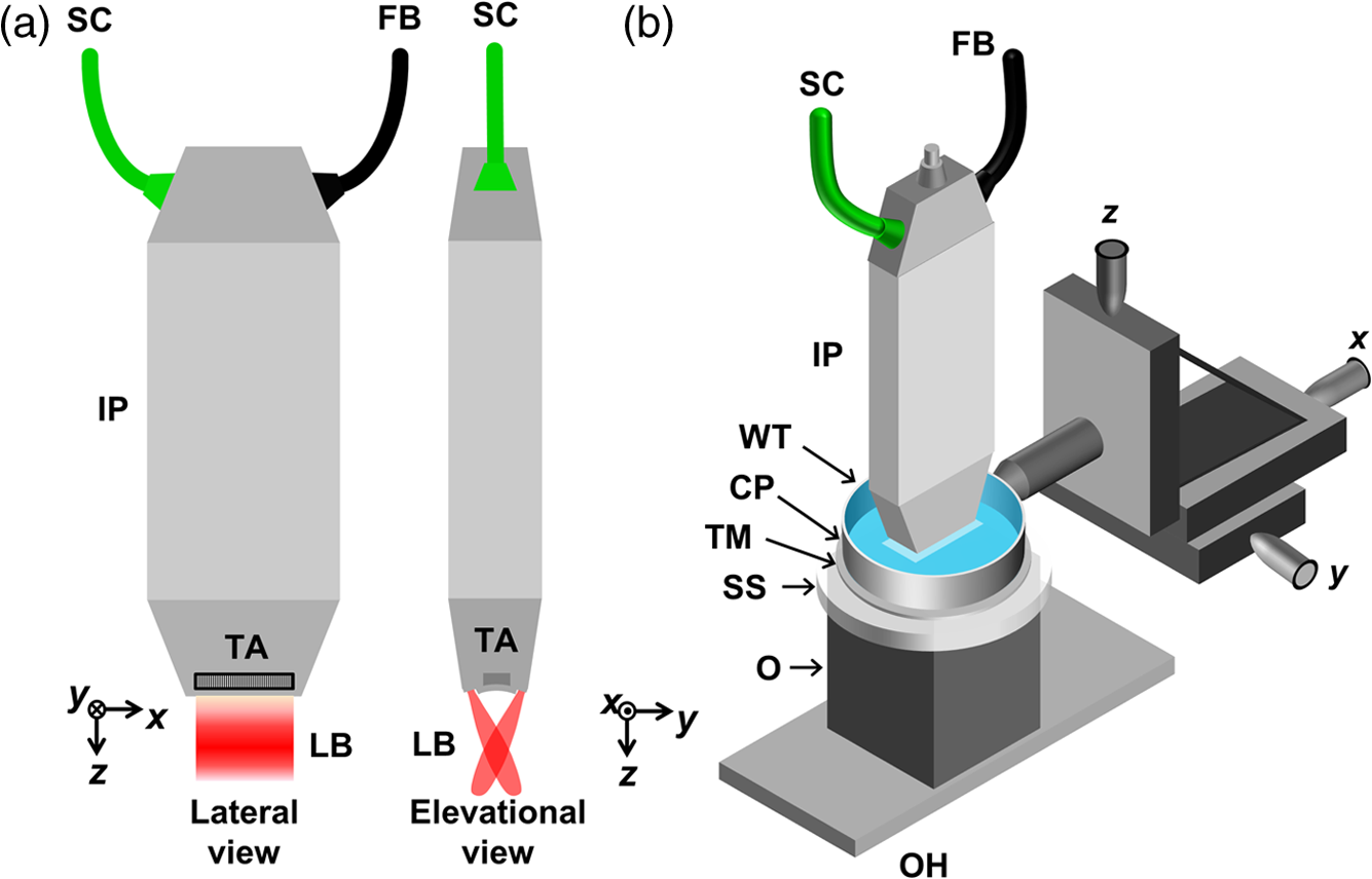

To obtain the Young’s modulus of the object, both the local stress and strain were measured in each experiment. After the compression plate contacted the stress sensor with a minimum load, a B-scan photoacoustic image of both the sensor and the object was obtained, from which the baseline thickness of the stress sensor $l_{\mathrm{b}}(x)$ was measured. Then, we exerted a small axial compression by moving the compression plate along the $z$-axis. After the object had stabilized, we obtained another B-scan photoacoustic image of the same cross section of the sensor and the object, from which the compressed thickness of the stress sensor $l_{\mathrm{c}}(x)$ was measured. The strain of the stress sensor ${ϵ}_{\mathrm{ss}}(x)$ at each lateral location was then calculated by

The local stress $\sigma (x)$ at each lateral position was obtained from the stress–strain curve of the sensor material [Fig. 2(a)], which was generated by an independent compression test. A 2-D short-window cross correlation between the two B-scan images was calculated to obtain a map of displacement. By numerically differentiating the displacement map, we obtained a strain image of the object ${ϵ}_{\mathrm{sa}}(x,z)$. The Young’s modulus value at each location $E_{\mathrm{sa}}(x,z)$ was then calculated by To ensure the accuracy of the Young’s modulus measurement, we first validated the stress measurement by the stress sensor. Placed on a high-precision digital weighing scale (S200, Ohaus), the stress sensor was imaged by QPAE before and after compression. The applied stress was calculated by where ${\sigma }_{\mathrm{A}}(x)$ is the compression stress, $g$ is the acceleration of gravity, $m_{\mathrm{a}}$ and $m_{\mathrm{b}}$ are the scale readings before and after compression, respectively, and $A$ is the area on which the compression force is applied. The local compression stress was also obtained by analyzing the photoacoustic images before and after compression with the method described above and averaged over the entire cross section. The stress measured by the stress sensor agreed well with the applied stress [Fig. 2(b)].

We first demonstrated the feasibility of QPAE by imaging agar phantoms with different concentrations. A small portion of black ink was mixed with the agar to provide optical absorption. Agar phantoms with concentrations of 20, 25, 30, 35, and $40\mathrm{g}/\mathrm{L}$ were embedded in gelatin at a concentration of $100\mathrm{g}/\mathrm{L}$. To mimic optical scattering in biological tissue, 1% intralipid was added to the agar phantoms and the gelatin background. The five phantoms were imaged by QPAE, and maps of Young’s modulus were obtained using the method described above [Figs. 3(a)–3(e)]. The entire cross sections of the five agar phantoms, with depths between 2.5 and 3.0 mm, were all clearly resolved by QPAE. Then, the Young’s modulus at each agar concentration was calculated by averaging over all the pixels with signal-to-noise ratios (SNRs) above 6 dB in the entire Young’s modulus map. Two methods were adopted to validate the Young’s modulus measurement in the phantoms. First, the averaged Young’s modulus values were fit to the following empirical relationship based on the agar concentrations¹⁹ [Fig. 3(f)]

where $E$ is the Young’s modulus at a given concentration $C$ and $k$ is a factor related to several parameters, including the molecular weight of agar used in the experiments and the agar mixing duration and temperature. The fitting results show a good agreement between the Young’s modulus measurement by QPAE and the empirical relationship based on the agar concentrations, with an $R^2$ value of 0.99. Second, the Young’s modulus measurements of the agar phantoms were validated by an independent standard compression test (SCT). In the SCT, stress–strain curves of the agar phantoms fabricated with the same procedure as above were generated. Young’s modulus values were calculated based on stress–strain curves with strain $<0.1$.²⁰ The Young’s modulus values of agar phantoms measured by QPAE agree well with those measured by SCT, further demonstrating the accuracy of QPAE in quantifying the absolute elasticity [Fig. 3(g)].

To demonstrate quantitative measurement of Young’s modulus in vivo, we imaged the right arm of a healthy human volunteer. All of the experiments were conducted in accordance with the human study protocols approved by the Institutional Review Board at Washington University in St. Louis. The biceps muscle was chosen because the volunteer would have sufficient control of the arm to avoid motion artifacts and could maintain the same arm position and same elbow angle of 90 deg throughout the experiment. The right arm was chosen to reduce the possible motion artifacts induced by the movement of the chest wall and the heart. During the experiments, the volunteer was asked to place his arm as flat as possible on the object holder. Then, he held a hand grip attached to a cable with different loadings pulling his arm straight but was tasked with keeping his elbow at a 90-deg angle during imaging. The stress sensor was placed on the biceps with ultrasound gel in between to keep good acoustic contact. The compression system and the photoacoustic imaging probe were on top of the stress sensor. Different loadings of 0.0, 2.5, 5.0, 7.5, and 10.0 kg were applied. At each loading, a B-scan photoacoustic image of a cross section of the stress sensor and arm was obtained first. In the B-scan photoacoustic image, three layers of structures were resolved, including the skin layer, the blood vessels, and a muscle layer [Fig. 4(a)]. Then, an axial compression force was exerted by moving the compression plate down along the $z$-axis. Another B-scan photoacoustic image of the same cross section of the stress sensor and arm was obtained. At each loading, a map of Young’s modulus was calculated based on the method described above [Figs. 4(a)–4(e)]. With QPAE, we were able to obtain the Young’s modulus values of the bicep up to 6-mm deep, within which the SNR was sufficiently high to calculate the displacements. We also calculated the averaged Young’s modulus values for each layer [Fig. 4(f)]. The skin had an average Young’s modulus value of 15.9 kPa, and we found that it stayed invariant with increasing loadings of the arm. The Young’s modulus of the muscle layer increased linearly with the loading applied. The result indicated that the elastic modulus of the biceps muscle has a linear relationship with the loading applied, which agrees with previous shear modulus measurements by MRE.²¹ A slight increase of the Young’s modulus was also observed in the cephalic vein, which possibly resulted from the increased blood supply to the arm due to repeated loading applied during the experiments. The in vivo results in human arm demonstrated the capability of QPAE in measuring the Young’s modulus quantitatively.

Note that in the phantom and in vivo experiments above, the maximum deformation of the phantom and the biological tissue was controlled to be smaller than 0.1. This ensures that the stress–strain response stayed in the linear range, so the Young’s modulus calculation was valid.²⁰ However, this requirement was not necessary for the stress sensor because we had characterized its stress–strain behavior with stain up to 0.5. The Young’s modulus was calculated only on the pixels with SNRs above 6 dB because the displacement calculation based on the cross correlation was only valid for pixels with SNRs above 6 dB.

The spatial resolutions of QPAE are $86\mu \mathrm{m}$ in the axial direction, $119\mu \mathrm{m}$ in the lateral direction, and $1237\mu \mathrm{m}$ in the elevational direction, determined by the linear-array-based photoacoustic imaging probe.²² The minimum detectable displacement is $18.3\mu \mathrm{m}$, which is determined by the data acquisition sampling rate of 84 MHz and the average speed of sound in biological tissue of $1540\mathrm{m}/\mathrm{s}$. The range of Young’s modulus measurement by QPAE depends on two factors. One is the range of strain measurement by PAE. The other is the ratio of the elasticity of the stress sensor to that of the object to be imaged. The maximum measurable Young’s modulus is determined by the maximum stress measured by the stress sensor and the minimum strain of the object to be imaged, and vice versa for the minimum measurable Young’s modulus. For a given stress sensor and PAE system, the maximum measurable Young’s modulus $E_{\max }$ is

where $d_{\min }$ represents the minimum detectable displacement in PAE, which is $18.3\mu \mathrm{m}$ in our system. The original object thickness $l$ is around 6 mm in the above experiments. The maximum measurable stress ${\sigma }_{\max }$ is theoretically limited to the stress, at which the sensor breaks down. In practice, if the stress sensor works in the linear stress–strain response range ($\text{strain}<0.1$), the maximum measurable stress for the sensor would be 3 kPa, resulting in a maximum measurable Young’s modulus of 983 kPa. If we reach a strain of 0.4 for the stress sensor, the maximum measurable Young’s modulus would be 28.3 MPa. The minimum measurable Young’s modulus $E_{\min }$ can be calculated by where $l_{\mathrm{ss}}$ represents the thickness of stress sensor and ${ϵ}_{\max }$ is the maximum strain of the object. For valid Young’s modulus calculation, the stress–strain response of the object needs to stay in the linear range; thus, the maximum strain of the object should be 0.1. For a 2-mm-thick stress sensor in our QPAE system, the minimum measurable Young’s modulus would be 3.2 kPa.

Surpassing conventional PAE, QPAE achieves quantification of absolute Young’s modulus instead of relative values by utilizing a piece of silicone rubber with known stress–strain behavior as a reference stress sensor. An important underlying assumption in QPAE is that the compression stress is uniform along each A-line (the depth). During the phantom and in vivo experiments, to maintain the validity of the assumption by eliminating boundary effects, the compression plate was made much larger than the object to be imaged. Although internal structures of the object can also affect the assumption, the method should remain sufficient for tissues with laminar structures, such as the skin and muscles.²³ To obtain more accurate results without the assumption of uniform stress along depth, an inverse problem for the three-dimensional distribution of stress within the object needs to be solved.²⁴

To the best of our knowledge, this is the first quantitative imaging of absolute elasticity in biological tissue by PAT. QPAE achieves mapping of the absolute Young’s modulus in vivo up to 6-mm deep, which is in the optical diffusive regime and thus enables longitudinal imaging of tissue elasticity. QPAE can be exploited for potential clinical applications, especially for long-term measurement of tissue elasticity such as monitoring softening of the cervix during pregnancy.