2.1.

Laser Speckle Contrast Imaging System

An LSCI system was designed and constructed specifically to examine the effects of the optical properties of the moving fluid on contrast values (Fig. 1). The system was essentially identical to the one used in Khaksari and Kirkpatrick.⁵ A polarized 660-nm diode laser (B&W Tek, Newark, Delaware) was used to illuminate a section of glass tubing with an outer diameter of 2 mm and an inner diameter of 1.5 mm resting on top of a grooved plastic base. The illuminated region was $\sim 20\mathrm{mm}$ in length. The glass tube, which served as our imaging window, rested in the groove. The glass tube was attached to a segment of rubber tubing that ran from the fluid phantom reservoir and through a miniperistaltic pump (Instech Laboratories, Plymouth Meeting, Pennsylvania, model P625) that controlled the flow velocity. The miniperistaltic pump was controlled by an Arduino microcontroller. A MATLAB^® GUI controlled the imaging CCD camera (Point Grey, Dragonfly, Vancouver, British Columbia, Canada) and the pump and also calculated and saved contrast images in near real-time.

Fig. 1

Diagram of the LSCI and flow systems. [Reproduced from Ref. 5].

2.2.

Liquid Phantoms

We used an added-absorber method to generate our flow phantoms. We initially created purely scattering phantoms in the same fashion as was done in Khaksari and Kirkpatrick⁵ by mixing calcium aluminum borosilicate glass microspheres (LUXSIL Cosmetic Microspheres, Potters Industries, Inc., Malvern, Pennsylvania) with de-ionized (DI) water. The microspheres were polydisperse in terms of diameter, ranging between 9 and $13\mu \mathrm{m}$, which is close to the diameter of red blood cells. The microspheres had mass density of $1.1\mathrm{g}/\mathrm{cc}$, which, being close to that of water, minimized settling. Using a Mie calculator,¹² the appropriate microsphere concentration was calculated using Mie theory to approximate the scattering coefficient of whole blood at various hematocrit levels.¹¹ For these calculations, we assumed that the microspheres were pure scatterers and that ${\mu }_{\mathrm{a}}=0$. These assumptions were made to more readily separate the combined effects of absorption and scattering. Furthermore, the absorption coefficient of the glass microspheres is negligible compared to the scattering coefficient at the wavelength of light employed, so the assumption is valid. Once the necessary concentrations of microspheres needed to create samples that approximate the scattering properties of whole blood were calculated, the flow phantoms were made by adding the calculated amount of microspheres to DI water. Ten solution phantoms of different scatterer concentrations were made using the results from the Mie calculations. Scattering coefficients of the fluid phantoms were confirmed via ballistic transmission measurements. A modified version of the Lambert–Beer law was used to calculate the scattering coefficient. Equations (3) and (4) summarize the approach

To calculate the reduced scattering coefficient, ${\mu }_{\mathrm{s}}^{\prime }$, we assumed scattering anisotropy of $g=0.9$ from the Mie calculations and

Because the microsphere powder was polydisperse in terms of diameter, ranging between 9 and $13\mu \mathrm{m}$, with a mean size of $11.7\mu \mathrm{m}$, according to the manufacturer, but with an unknown size probability distribution, Mie calculations were performed assuming monodispersions of 9.0, 11.7, and $13.0\mu \mathrm{m}$. The scattering coefficients calculated via Mie theory were compared to the values generated via the ballistic transmission experiments in order to better characterize the scattering behavior of the fluid phantoms.

The effect of varying ${\mu }_{\mathrm{a}}$ on LSCI was also of interest in this study. Thus, a series of absorbing liquid phantoms was constructed. An “added-absorber” approach was followed in making these phantoms. Empirically determined volumes of India ink were added to the purely scattering phantoms and pure DI water. Using ballistic transmission again, and with a priori knowledge of the scattering coefficient of the sample, the absorption coefficient was estimated as

2.3.

Laser Speckle Contrast Imaging Measurements

Each fluid phantom was imaged with the LSCI system described above at a uniform velocity. Figure 2 shows the cross-section of the sample preparation we used in the LSCI setup. As can be seen in the figure, the moving and static parts are in the same depth of field (flow is coming out of the page, toward the reader).

Fig. 2

Sample cross-section. [Reproduced from Ref. 5].

The camera lens (100 mm macrozoom) was fixed at $f/32$, which resulted in relatively large speckles (see below) and an extended depth of field. During the experiments, all experimental parameters were held constant with the exception of the optical properties of the moving fluid, which varied by sample. The flow velocity was held constant at $5\mathrm{mm}/\mathrm{s}$. The camera integration time was 6 ms and held constant for all the experiments. Images were acquired at a frame rate of $125\text{frames}/\mathrm{s}$. Thus, the only varying parameters were the optical properties of the fluid phantom used.

An important parameter in an LSCI experiment is the relative size of the speckles versus camera pixel size.¹³ The minimum speckle size (in pixels), ${\sigma }_{\min }$, was determined by calculating the power spectral density of the raw speckle images [Figs. 3(a) and 3(b)] and applying Eq. (8)

Fig. 3

(a) A laser speckle pattern, (b) power spectral density of the speckle pattern shown in (a). The diameter of the bright central region is inversely proportional to the minimum speckle size in the speckle pattern.

In LSCI, unlike other speckle techniques, such as diffusing wave spectroscopy, the minimum speckle size should not match the camera pixel size but must be greater than two times of camera pixel pitch to meet the spatial Nyquist criteria.¹³ In these experiments, the minimum speckle size was set to 2.72 times the pixel size ($10.7\mu \mathrm{m}$). The minimum speckle size in the image plane was, therefore $\approx 29.1\mu \mathrm{m}$. It was also ensured that the speckle size relative to the size of the sliding window used in the contrast calculations ($7\times 7\text{pixels}$) was appropriate to account for the local statistics of the calculated contrast.⁴

For image collection, the laser was set slightly off-axis to avoid specular reflection. A video of 100 frames was recorded with the CCD camera for each sample. The experiment was repeated three times for each sample. In the end, 300 frames of raw speckle and 300 contrast images were recorded for each sample. The 300 frames were then averaged to create an “average” contrast image. The ratio between the dynamic (fluid) region and the static region ($K_{\text{ratio}}$) of the contrast images was calculated for all of the images. Similar to above, an $11\times 11$ matrix was created of $K_{\text{ratio}}$ values. This matrix demonstrated the change in contrast that resulted from the change in the optical properties of the fluid phantoms. The numerical values of $K_{\text{ratio}}$ lay between 0 and 1.0, since the contrast is always lower in the fluid (dynamic) region of the contrast image

3.1.

Phantom Characterization

The scattering coefficients for 10 different sample concentrations of microspheres (plus pure DI water) was measured and by assuming $g=0.9$, the reduced scattering coefficient of the samples was estimated. By increasing the number of scatterers, the reduced scattering coefficient increased in a linear fashion. Figure 4 shows the phantom’s reduced scattering coefficients and the relationship between the concentration of scatterers and the reduced scattering coefficient. Because the microspheres were polydisperse with an unknown size distribution, Fig. 4 also displays the results of Mie scattering simulations for the minimum, maximum, and mean sizes of the spheres as reported by the manufacturer. It is seen that the polydisperse mixtures displayed overall scattering behavior similar to that of a monodisperse system of $\sim 10.5\mu \mathrm{m}$ spheres. Microsphere concentration [$c$] ranged from $9.2\times {10}^{-3}\mathrm{mg}/\mathrm{ml}$ ($1\times {10}^{-5}\text{spheres}/{\mu \mathrm{m}}^3$) to $9.2\times {10}^{-2}\mathrm{mg}/\mathrm{ml}$ ($1\times {10}^{-4}\text{spheres}/{\mu \mathrm{m}}^3$), and the reduced scattering coefficient of the samples ranged from 0.48 to $4.84{\mathrm{mm}}^{-1}$. A linear regression through the experimental data yielded the following relationship:

Fig. 4

Mie calculations predicting the reduced scattering coefficient for glass spherical particles of 9.0, 10.5, 11.7, and $13.0\mu \mathrm{m}$ diameters (dashed lines, red dashed lines online). Reduced scattering coefficient as determined by ballistic transmission data points is shown for the fluid phantoms (dots) along with the best-fit line in a least-squares sense. The polydisperse microsphere phantoms behaved approximately as a monodisperse system made of $10.5\mu \mathrm{m}$ glass microspheres. (${\mu }_{\mathrm{s}}^{\prime }=48.66[c]-0.196$; $r^2=0.98$.)

Fig. 5

Plot of the absorption coefficient of the fluid phantoms as a function of India ink concentration. ${\mu }_{\mathrm{a}}=367.3[\mathrm{ink}]+.0016$; $r^2=0.996$).

3.2.

Contrast Imaging

The main goal of this investigation was to examine the combined effects of scattering and absorption on the contrast in LSCI images. As discussed above, the experiments were run for the 121 phantoms with unique combinations of reduced scattering and absorption coefficients. Accordingly, within the matrix, the absorption coefficient changed when moving along the rows and the reduced scattering coefficient changed moving along the columns. Values of $K_{\text{ratio}}$ were obtained from this matrix, and the contrast ratios for the different combinations of optical properties were plotted.

Figure 6 shows an example LSCI images from the $11\times 11$ $K_{\text{ratio}}$ matrix. The tubing that contained fluid phantom flowed runs from the lower left to the upper right and the resulting low-contrast area is readily observed in the images. The triangular regions to the right and left of the tube are the “static” plastic block.

The relationship between $K_{\text{ratio}}$ and ${\mu }_{\mathrm{s}}^{\prime }$ was found to be linear. An increase the concentration of scatterers [$c$], which manifested as an increase in ${\mu }_{\mathrm{s}}^{\prime }$ resulted in a decrease in $K_{\text{ratio}}$.⁵ The results are plotted in Fig. 7, where $K_{\text{ratio}}$ is plotted as a function of ${\mu }_{\mathrm{s}}^{\prime }$ for 11 different values of ${\mu }_{\mathrm{a}}$. All the linear fits were statistically significant ($t$-test, $p<0.05$); the slopes, $m_{\mathrm{s}}$, of the best fit lines ranged between $-0.072\frac{\mathrm{\Delta }{K}_{\text{ratio}}}{\mathrm{\Delta }{\mu }_{\mathrm{s}}^{\prime }}\le m_{\mathrm{s}}\le -0.05\frac{\mathrm{\Delta }{K}_{\text{ratio}}}{\mathrm{\Delta }{\mu }_{\mathrm{s}}^{\prime }}$; and there was no significant difference between the slopes ($t$-test, $p<0.05$). The mean slope was $-5.53\times 10{}^{-2}\frac{\mathrm{\Delta }{K}_{\text{ratio}}}{\mathrm{\Delta }{\mu }_{\mathrm{s}}^{\prime }}$. Figure 8 plots the $y$-intercepts (${\mu }_{\mathrm{s}}^{\prime }=0$) of the regression lines shown in Fig. 7 as a function of absorption coefficient, ${\mu }_{\mathrm{a}}$. This plot reveals a linear reduction in $K_{\text{ratio}}$ with an increase in ${\mu }_{\mathrm{a}}$ in our experiments ($K_{\text{ratio}|{\mu }_{\mathrm{s}}^{\prime }=0}=-5.68{\mu }_{\mathrm{a}}+0.94$; $r^2=-0.982$).

As will be discussed below, this reduction in contrast is due to the attenuation of the light reaching the static scattering block below the moving fluid and, thus, reducing the influence of these static scatterers on the overall contrast. Others^8,9 have observed an increase in contrast with an increase in absorption; however, in their experiments, there was no underlying layer of static scatterers and their scattering mediums were optically semi-infinite or close to it.

Fig. 6

A representative LSCI image. The fluid motion was in the low contrast region flowing from lower left to upper right of the image. The surrounding higher contrast triangular areas are the static plastic block.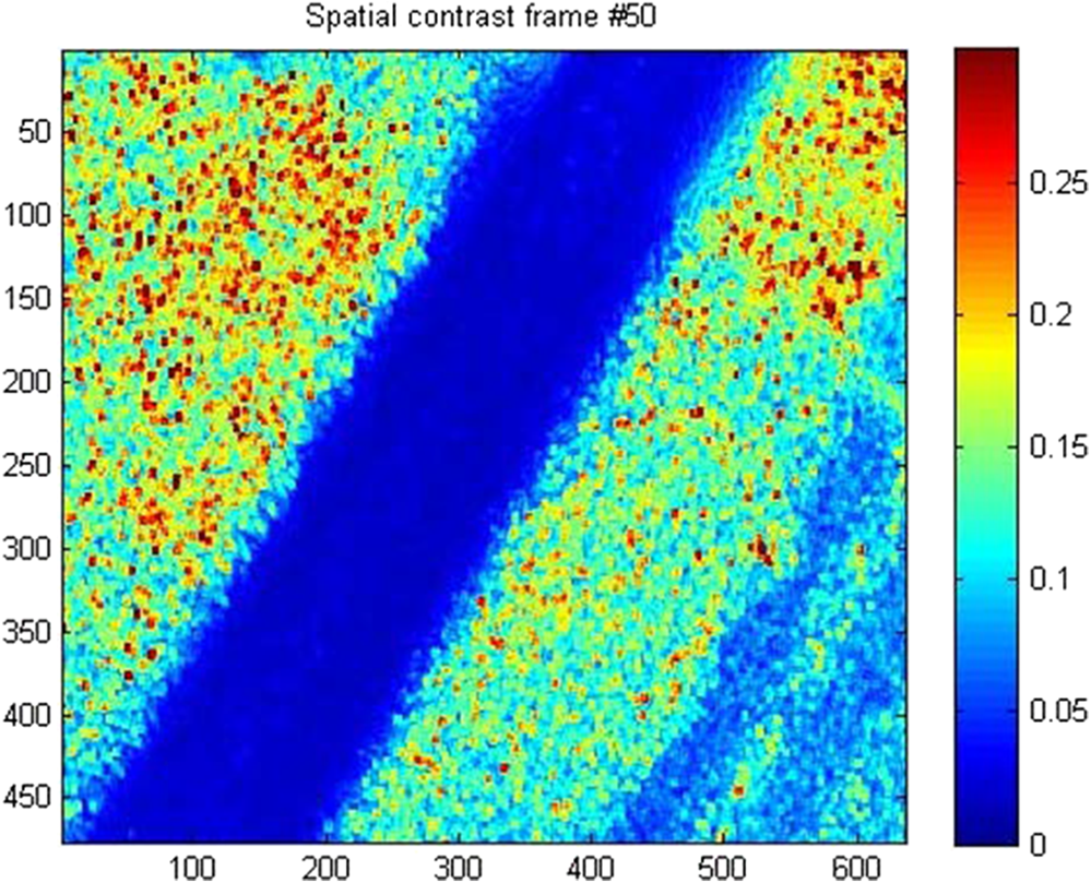

Fig. 7

Plot of $K_{\text{ratio}}$ versus ${\mu }_{\mathrm{s}}^{\prime }$ at 10 different values of ${\mu }_{\mathrm{a}}$. All slopes were statistically significant ($t$-test, $p<0.05$) and there was no statistically significant difference between the slopes ($t$-test, $p<0.05$). The mean slope was $-5.53\times {10}^{-2}\frac{\mathrm{\Delta }{K}_{\text{ratio}}}{\mathrm{\Delta }{\mu }_{\mathrm{s}}^{\prime }}$. Absorption coefficient is lowest for the top line and highest for the bottom line.

Fig. 8

Plot of the $y$-intercepts (${\mu }_{\mathrm{s}}^{\prime }=0$) of Fig. 7 as a function of respective absorption coefficients. An increase in absorption resulted in a linear decrease in $K_{\text{ratio}}$ in these experiments due to reducing the influence of the underlying static scatterers. (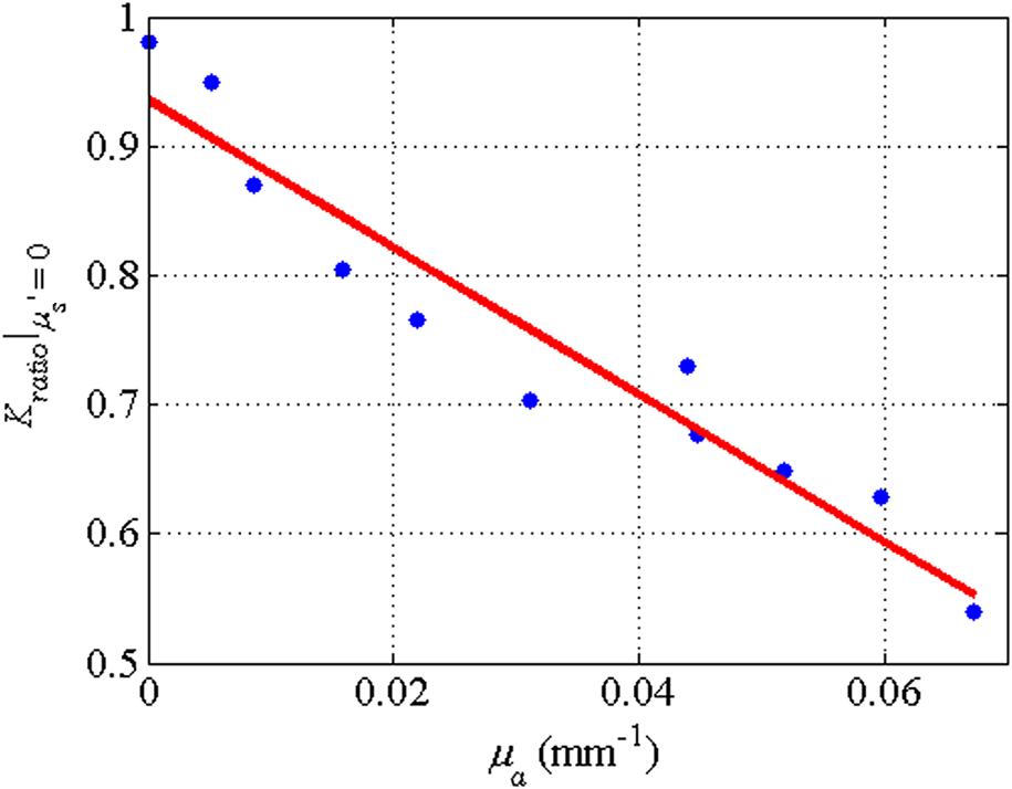$K_{\text{ratio}|{\mu }_{\mathrm{s}}^{\prime }=0}=-5.68{\mu }_{\mathrm{a}}+0.94$; $r^2=-0.982$).

Thus, with an increase in absorption coefficient, $K_{\text{ratio}}$ decreased. This trend is shown for the fluid phantoms with 11 different reduced scattering coefficients in Fig. 9. All the linear fits were statistically significant ($t$-test, $p<0.05$); the slopes, $m_{\mathrm{a}}$, of the best fit lines ranged between $-3.52\frac{\mathrm{\Delta }{K}_{\text{ratio}}}{\mathrm{\Delta }{\mu }_{\mathrm{a}}}\le m_{\mathrm{a}}\le -4.55\frac{\mathrm{\Delta }{K}_{\text{ratio}}}{\mathrm{\Delta }{\mu }_{\mathrm{a}}}$; and there was no significant difference between the slopes ($t$-test, $p<0.05$). The mean slope was $-4.01\frac{\mathrm{\Delta }{K}_{\text{ratio}}}{\mathrm{\Delta }{\mu }_{\mathrm{a}}}$. Figure 10 plots the $y$-intercepts of these regression lines as a function of the corresponding reduced scattering coefficients. This plot reveals a linear reduction in $K_{\text{ratio}}$ with an increase in ${\mu }_{\mathrm{s}}^{\prime }$ in our experiments [$K_{\text{ratio}|{\mu }_{\mathrm{a}}=0}=(-7.02\times 10{}^{-2}){\mu }_{\mathrm{s}}^{\prime }+0.92$; $r^2=-0.976$].

By combining the scattering and absorption data, the influence of total attenuation coefficient, ${\mu }_{\mathrm{t}}={\mu }_{\mathrm{s}}^{\prime }+{\mu }_{\mathrm{a}}$, on $K_{\text{ratio}}$ was assessed. As expected from the results presented above, there was a linear decrease in $K_{\text{ratio}}$ with an increase in ${\mu }_{\mathrm{t}}$. Figure 11 shows the results of the $K_{\text{ratio}}$ versus ${\mu }_{\mathrm{t}}$ for the samples that were along the major axis of the scattering—absorption phantom matrix. The equation describing the least-square fit was $K_{\text{ratio}}=-0.14{\mu }_{\mathrm{t}}+0.93$; $r^2=-0.94$. The slope is statistically significant ($t$-test, $p<0.05$).

Fig. 9

Plot of $K_{\text{ratio}}$ versus ${\mu }_{\mathrm{a}}$ at 10 different values of ${\mu }_{\mathrm{s}}^{\prime }$. All slopes were statistically significant ($t$-test, $p<0.05$), and there was no statistically significant difference between the slopes ($t$-test, $p<0.05$). The mean slope $-4.01\frac{\mathrm{\Delta }{K}_{\text{ratio}}}{\mathrm{\Delta }{\mu }_{\mathrm{a}}}$. Scattering coefficient is lowest for the top line and highest for the bottom line.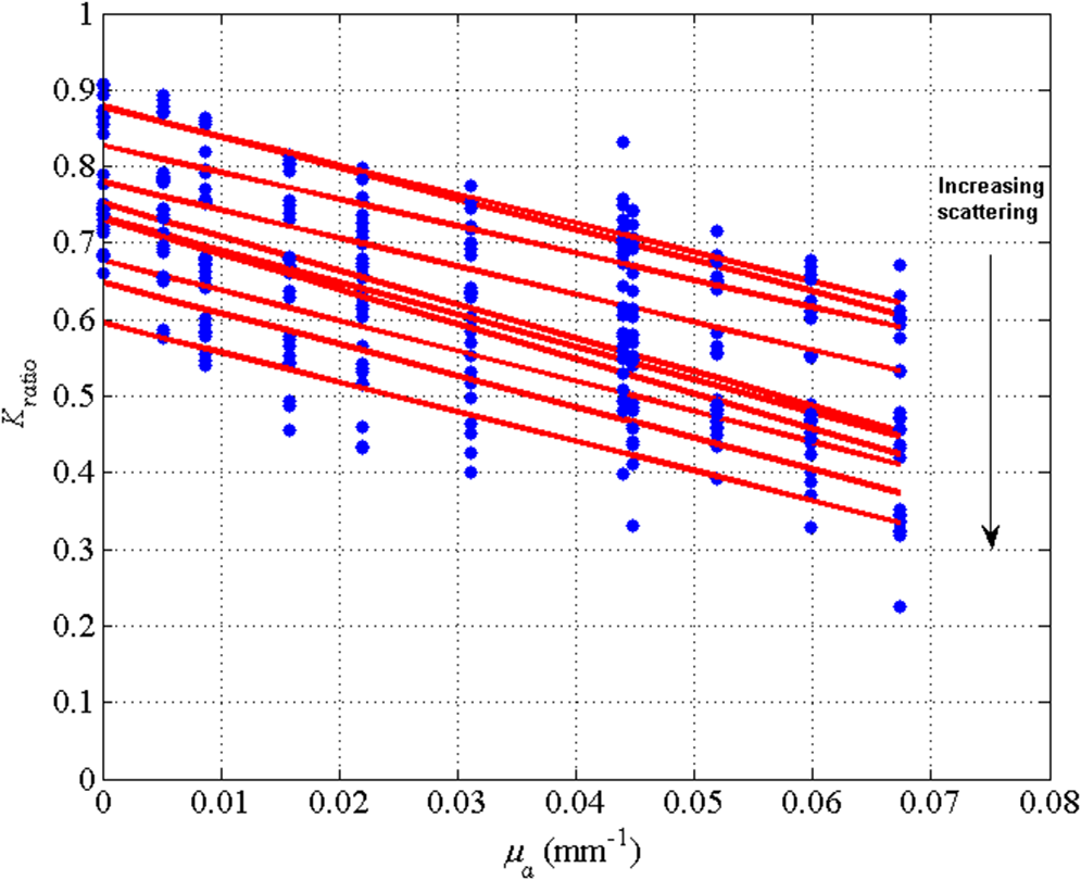

Fig. 10

Plot of the $y$-intercepts (${\mu }_{\mathrm{a}}=0$) of Fig. 7 as a function of respective reduced scattering coefficients. An increase in scattering resulted in a linear decrease in $K_{\text{ratio}}$. ($K_{\text{ratio}|{\mu }_{\mathrm{a}}=0}=(-7.02\times 10{}^{-2}){\mu }_{\mathrm{s}}^{\prime }+0.92$; $r^2=-0.976$).

Fig. 11

Plot of $K_{\text{ratio}}$ versus ${\mu }_{\mathrm{t}}$ for the phantom samples that were along the major axis of the scattering and absorption phantom matrix. An increase in ${\mu }_{\mathrm{t}}$ resulted in a significant decrease in $K_{\text{ratio}}$. ($K_{\mathrm{ratio}}=-0.14{\mu }_{\mathrm{t}}+0.93$; $r^2=-0.94$).