|
|
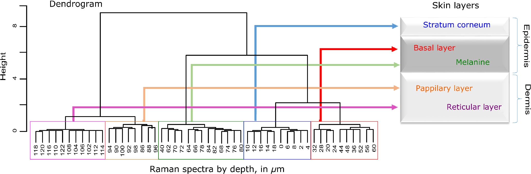
1.IntroductionUnderstanding in vivo systems is the main focus of the life and applied sciences. Biological systems show dynamic behavior and have a diversified biochemical constitution. These systems often interact with various exogenous agents like the interactions of the biochemicals that are being monitored with other compounds present in the body (other biochemicals common to the tissue in question, drugs, and so on) and the interactions with the various external environmental parameters like humidity, temperature, and sunlight. These interactions will add to their complex nature. Despite the complexity, which is a characteristic inherent of these systems, various in vivo applications corroborate as effective and early diagnostic tools to explain the mechanisms of action of these external agents. In the field of in vivo research, spectroscopic techniques have an important role to play owing to their fast and nondestructive analysis of biological data. Many studies have reported that the Raman spectroscopy is a powerful tool in biological, diagnostic, forensic, and pharmaceutical areas.1–5 Raman spectroscopy provides a highly sensitive approach to analyze the subtle molecular (biochemical) changes6 taking place in these in vivo systems. Advances in Raman spectroscopy allow the use of more versatile equipments for in vivo analysis without loss of quality information.7 Nowadays, the techniques used for in vivo applications have high sensitivity and this characteristic can lead to many difficulties in the interpretation of results. For example, samples of urine, plasma, saliva, or biological tissues when analyzed using spectroscopic techniques provide many variables that refer to the complex biochemical composition of each sample. Other difficulties are related to spectral overlapping, interference, and presence of a large number of biochemical compounds to analyze. To overcome these difficulties, the chemometric approach is often used with various multivariate statistical tools like principal component analysis (PCA),8,9 partial least squares (PLS),10,11 orthogonal signal correction (OSC),12,13 orthogonal PLS (OPLS),14 discriminant analysis (DA),15,16 and hierarchical cluster analysis (HCA)17,18 in the vibrational spectroscopic techniques19 for the interpretation of experimental data. Some of these in vivo works combine Raman spectroscopy with these multivariate analyses. Kendall et al.20 used a model of discriminant classification for the prediction of tissue pathology from the measurements of Raman spectra. Similar analyses were used to study prostate cancer,21 brain tissue,22 and skin lesions.23 The use of PCA with Raman spectroscopy to differentiate various kinds of cancer cell populations was proposed by Krishna et al.,24 and a similar approach was used to study the composition of human tear fluid by Filik and Stone.25 Various applications of Raman spectroscopy with the chemometric approach were reported in the literature.26–31 However, in all these previously reported studies, the statistical methodology that was used to interpret the spectra was not given its due importance and often restricted to a mere mention of the names of various statistical tests used. Among the various biological systems, human skin presents a lot of variations owing to its complex nature. In addition to this, the complexity is further increased with the use of the confocal Raman technique as this technique allows the analysis of various skin layers in a single study. Furthermore, the interpretation of the Raman data of human skin has not yet been completely understood. In view of this, the search for vibrational markers that discriminate groups of samples in confocal Raman spectroscopy is not trivial. For this, we present certain methods that can be implemented in the studies applying confocal Raman spectroscopy for biological samples. Therefore, the main focus of this work is to avail various statistical approaches to explore vibrational markers related to skin aging for an in vivo human skin study applying confocal Raman spectroscopy. This work presents even minute details of these statistical approaches including step-by-step explanation of univariate (parametric and nonparametric) and various multivariate analytical tools like HCA, PCA, and PLS-DA to understand the vibrational markers related to skin aging. This paper mainly contributes to the discussions in the area of human skin research by confocal Raman but can be extended to a large research community that uses other kinds of biological samples. In order to have a proper understanding of the application of these methods, Appendix material is attached which explains complete routine of data analysis using free R software.32 2.Materials and Methods2.1.Samples: Selection of VolunteersFor this study, volunteers with skin phenotypes I and II according to Fitzpatrick classification33 were selected. Volunteers with presence or history of irritation, sensitivity to cosmetics, dermatological diseases, and those who used cream cosmetics over the past 48 h preceding this examination were excluded from the study. Prior approval from the Research Ethics Committee was obtained for this study (report number 132.812). This study involves confocal Raman measurements of skin of 30 female participants segregated into three groups on the basis of age and presence of diabetes mellitus type II as young healthy (YH), elderly healthy (EH), and elderly diabetic (ED). YH contains the volunteers in the age group of 20 to 30 years, whereas EH and ED groups include the volunteers in the age group of 56 to 81 years. This article aims to determine the vibrational markers indicating intrinsic skin aging by comparing the sets of samples of young and elderly volunteers. The process of skin aging can be studied from the changes in the biochemical composition of the dermis layer of the skin, as it is mainly represented by the degradation of collagen present in this dermis layer. The ED group was included in this study as diabetes mellitus causes an acceleration in the aging process due to the glycation process. Therefore, the changes due to intrinsic aging would be enhanced in this group. In this research group, there is an advanced glycation end products (AGEs) overload in skin tissue, degrading the framework formed by the amino acids of type I collagen such as proline (P) and hydroxyproline (HP).34,35 These diabetic people have three times more Amadori products (precursors of AGEs) and twice more AGEs than normoglycemic people. Furthermore, independent authors use this group of volunteers to assess extreme conditions in aging of adipose tissue36 and other diagnostics.37 Therefore, in the volunteers with diabetes mellitus, the variability is expected to be high owing to the rapid rate of skin aging caused by the glycation process. 2.2.Study ConditionsThe instrumental technique described here is noninvasive and presents no risk of causing any damage to the volunteer. Before starting the skin measurements, the volunteers were acclimatized to temperature and relative humidity for 60 min. After acclimatization, the volunteers were seated with the forearm positioned on an aluminum plate, which contains an optical window. Before collection of Raman spectra, the forearm sites used for the measurements were cleaned with cotton soaked in 1.0 mL of ethyl alcohol 97%. 2.3.InstrumentationThe acquisition of confocal Raman spectra of human skin was performed using a confocal Raman system (River Diagnostics, Model 3510 skin composition analyzer) coupled to a laser with exciting radiation of wavelength 785 nm. The laser light is focused on the skin with a microscope lens () located under a quartz window. The Raman signal is collected by a charge coupled device (CCD) and recorded on a computer connected to this system. The calibration of wavelength was performed by using lines of a neon–argon lamp. The laser power utilized for skin analysis was 27 mW. 2.4.Study DesignThe measurements were performed on the forearm of the volunteers. The specific and selected regions of forearm were exposed to the laser light from the objective. The scattered laser light was collected by the same objective and sent to the spectrophotometer after being filtered. The data were collected in a spectral range 400 to with spatial resolution of and two accumulations by spectra. The objective used is coupled to a piezoelectric system that controls the depth of the focal plane. Raman spectra were acquired from the surface of skin up to a depth of . Confocal Raman spectra were recorded in different tracks with varying step sizes. Steps of for the first depth, then with a step size of in the region from 20- to depth, and finally with a step size of in the region from 60- to depth. In total, 52 spectra were recorded from each volunteer. The exposure time for the first two tracks, i.e., from surface to and 20 to , was 10 s. For the higher depths greater than , the exposure time was increased to 60 s. This is due to the fact that the number of photons that reaches the detector will be reduced in these higher depths. In the preliminary tests, with this exposure time, spectra of the dermis region were obtained with good quality and high signal-to-noise ratio. 2.5.Preprocessing of DataTo minimize the influence of noise, the spectra were smoothed by Labspec software (Horiba JobinYvon, France) using Savitzky–Golay filter (grade 2, size 3). Using the same software, fluorescence present in the data was eliminated by subtracting a baseline using the line segments between the wavenumbers: 400, 470, 552, 588, 633, 794, 798, 994, 1144, 1495, and . The specific noise coming from cosmic rays (CRs) was eliminated through a specific feature of this software. CRs occasionally affect CCD detectors, introducing large spikes with very narrow bandwidth in the spectrum and can occur randomly in the spectra at various wavenumber positions. These spikes should be removed in order to nullify its influence on the normalization and statistical analysis of data.38 Spikes can be visually detected in the Raman spectrum because of its characteristic of having positive peaks with high intensity values with bandwidth much narrower than Raman bandwidth. Following this subtraction, the spectra were normalized by vector normalization, in which each Raman intensity was divided by square root of sum of the squared intensities calculated using the full spectrum.39,40 After these procedures, the preprocessed spectra were subjected to statistical analysis. 3.Statistical Analysis of Data3.1.Cluster Analysis: Selecting the Correct Skin LayerBefore starting statistical analysis of the differences in confocal Raman spectra for the groups of samples, it should be ensured that the comparisons between the groups are made using the same layer of the skin. Confocal Raman system acquires the spectra at different depths of the skin. Therefore, it is necessary to know which set of spectra corresponds to what layer of the skin. In order to identify and separate the different layers of the skin, an exploratory analysis by the HCA was performed on a single sample containing spectra varying in depth. This is necessary to select which skin depth will be used for the subsequent discussion of the study. Cluster analysis is one of the important techniques for pattern recognition. It finds “natural” grouping (unsupervised) based on the similarity of the intensities of the dataset variables. It is applied when the spectra are to be interpreted as members of a category like skin depth. An excellent visualization of these clusters by similarity is dendrograms, also called the tree of clusters. Figure 1 shows the dendrogram of the HCA for human skin according to the different depths obtained by confocal Raman equipment. By HCA, it is possible to classify the different layers of the skin into separate clusters. From these clusters, the set of spectra that corresponds to the skin layer to be monitored can be selected. In addition to the classification of spectra corresponding to various skin layers, cluster analysis is also useful to detect outliers. Forming a cluster with only one or two spectra or a distant cluster to others is a strong indication of anomalous data. In this case, the spectrum of this sample should be inspected to detect the possible error. Based on the inspection of the spectra, decision has to be made either to reprocess that spectrum or to repeat the experiment if possible or to reject that particular spectrum. There are some approaches for outlier detection such as Hotelling T, Mahalanobis distance, and Chi-square distribution.39,41 However, it is highlighted that it is not acceptable to remove any sample simply by considering it as an outlier. Outliers can be legitimate observations and sometimes very interesting and important details can be revealed by them. Therefore, it is very important to investigate the nature of the outliers before making a decision on their exclusion. From this study, the dermis region was chosen for further analysis as skin aging is mainly represented by the glycation and degradation of proteins like type I collagen present in the dermis region of the skin. Out of 52 spectra obtained per volunteer, spectra representing the dermis layer of each volunteer that were classified by cluster analysis were used for further analysis. The number of spectra of dermis region was found to be 30 per volunteer by cluster analysis. Average spectra calculated from these 30 spectra of dermis region for each individual were used in univariate and multivariate analyses. 3.2.Correlation Matrix: Representativity and Reproducibility of the StudyAn issue in academia is the representation of groups and volunteer numbers used for in vivo studies for the reproducibility of results. These issues must be addressed in studies using confocal Raman spectroscopy as these measurements can be questioned since each measurement is collected in a focal plane within specific surface area by the lens used. However, this issue of confocal Raman spectroscopy can be dealt with in many ways such as by assessing the changes in analytical information with depth and by determining the intragroup and intergroup correlations. The Pearson correlation matrix provides an easy interpretation of correlation between two measurements. This matrix considers each spectrum as a variable and calculates the correlation coefficient on a scale ranging from to . The data can be with high negative correlation (), with no correlation (zero), or with strong positive correlation (). This correlation coefficient is calculated from the mean and standard deviation of the observations given by the intensity at each wavenumber in the spectra. Figure 2 shows an example in which the Pearson correlation matrix can be used. This array has arranged three spectra at different depths in the dermis of 70, 93, and and compared them with the average spectrum calculated by taking the average of all the spectra that make up the layer of the dermis. It is very common to use the average of a set of spectra to plot a graph representing that set of spectra. The Pearson correlation array can be used to compare the correlation between two individual spectra as well as with the average of that set of spectra. Fig. 2Pearson correlation matrix. The range of the scale from high-negative correlation ( with red), uncorrelated (0 with white), to strong positive correlation ( with blue). 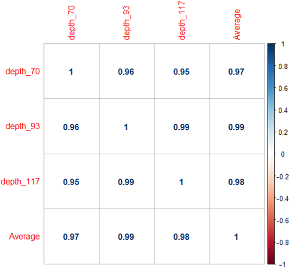 The analysis of Fig. 2 shows that the lowest correlation occurs for spectral comparison between the depths of 70 and (). This is expected because spectra are taken from the initial and terminal portions of the dermis, where there is high biochemical variability in the composition of the skin. However, since both these spectra belong to the basal layer, significant correlation has been observed even though there are certain differences due to variable skin composition. The same explanation applies for the comparison of the average of all the spectra from dermis with the individual spectra shown in Fig. 2. All the spectra show a strong positive correlation indicating that there is not much deviation from the average. Therefore, the average can be used to express the overall behavior of this layer. 3.3.Univariate and Multivariate Statistical Approaches: Revealing Vibrational MarkersOnce the adequate range of depth to analyze was assessed by HCA and correlation of individual spectra at different depths compared with the average spectrum used to represent the dermis by the Pearson correlation matrix, statistical data analysis starts the search for the spectral regions that can be used as an individual group with characteristics as relevant as possible with respect to the vibrational ways that discriminate the groups. Figure 3(a) shows the average spectra of dermis of each volunteer (average between the spectra collected in the range from 60- to depth) of the total of 30 volunteers in this study, and Fig. 3(b) shows the average of the average spectra of the dermis region of the volunteers belonging to the three groups, namely YH, EH, and ED. Figure 3(b) also gives the information on the residual spectra obtained upon comparing YH, EH, and ED groups. From the visual inspection of the average confocal Raman spectra and the residual spectra in Figs. 3(a) and 3(b), it is quite evident that it is not possible to clearly distinguish a spectral region capable of discriminating the three groups of volunteers analyzed. Fig. 3Raman spectra of human skin: (a) average dermis spectra of 30 volunteers and (b) average dermis confocal Raman spectra of young healthy (YH), elderly healthy (EH), and elderly with diabetes mellitus (ED) with the residual spectra obtained for the comparisons: ED minus YH, ED minus EH, and EH minus YH. 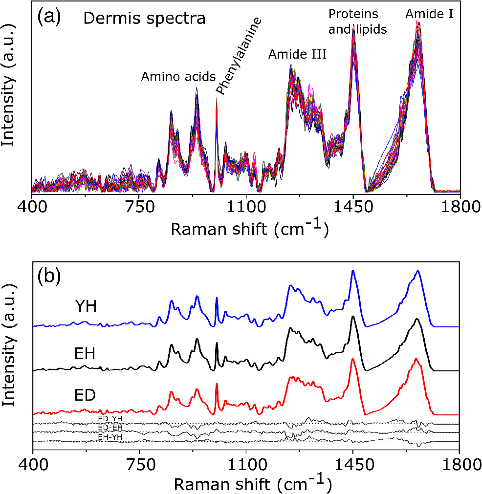 Different statistical approaches can be used to seek the spectral regions that are significant enough to describe the differences among the groups analyzed. These spectral regions indicate the vibrational markers responsible for explaining skin aging. In this study, we describe the steps used by both univariate and multivariate statistical approaches to explore these vibrational markers. These approaches can be used either alone or concomitantly as a result of their complementary character. In univariate statistical application on the set of spectra, each variable, i.e., each wavenumber, is analyzed separately. The sequence for this analysis is made variable by variable. In a multivariate approach, dimension reduction methods will be used and the spectral data are interpreted as a data matrix. In the case of nonsupervised analysis, the experiment corresponds to an array and by applying matrix algebra methods, the spectral regions that have greater variation in the data are determined, giving little importance to spectral overlap and noise regions. In the case of supervised analysis, only the regions correlated with a property of interest have more importance. Irrespective of the approach, all the wavenumbers that contribute are considered in a multivariate model with different weights. Figure 4 represents the flowchart of steps in statistical data analysis. Univariate analysis is performed by applying a set of hypotheses tests. The hypotheses tests consist of a statistical procedure based on probability theory in which a parameter is tested on a set of values. Two hypotheses are considered: the null hypothesis (to be tested) and the alternative hypothesis that will be accepted if the group does not fall within the tested null hypothesis. The decision whether the test set belongs to or can be made through the analysis of -values. It is important to note that for the correct application of hypothesis testing, the verification of the assumptions should be performed. If the assumptions are not checked properly, it may result in an incorrect inference about the dataset analyzed. For the univariate analysis, there is a great distinction between the sequence of processes to be employed if the data follow a normal distribution (parametric statistics) or not (nonparametric statistics). The univariate approach begins with checking the normality of the data. If the data show the normal Gaussian distribution pattern, then it follows the path of parametric analysis; otherwise, it will follow nonparametric analysis. In the scheme shown in Fig. 4, Lilliefors test was used for the normality check.42 In this case, the default null hypothesis, which states that the sample follows normal distribution, is tested against the alternative hypothesis stating that it does not follow normal distribution. The nonparametric test used was the Kruskal–Wallis test.43 This test compares the medians of the samples and gives the -value for the hypothesis testing. Null hypothesis indicates that all the samples are drawn from the same population, whereas the alternative states that they are from different populations. The test for the homogeneity of variances is the F-test.44 An F-test of the null hypothesis checks that two independent samples coming from normal distributions are with the same variance against the alternative hypothesis, which states that they came from normal distributions with different variances. -Test44 was used to check if the average of the intensities of the tested groups is the same or different. -Test of null hypothesis checks that the data in independent random samples from the normal distributions are with equal averages against the alternative hypothesis stating that the averages are not equal. The complete sequence shown in Fig. 4 can be implemented in free R software, which is presented in the Appendix and discussed in detail in various statistics books.43,44 The -value analysis for a given level of statistical significance is used to infer whether a variable is significant or not. This result is usually disposed in a table of -values for each wavenumber. However, it is possible to make a -value graph to facilitate the visualization of the results (as shown in Fig. 5). Fig. 5Results of univariate analysis for young healthy (YH), elderly healthy (EH), and elderly with diabetes mellitus (ED). are represented by black stars, and are represented by open circles. Horizontal line represents . 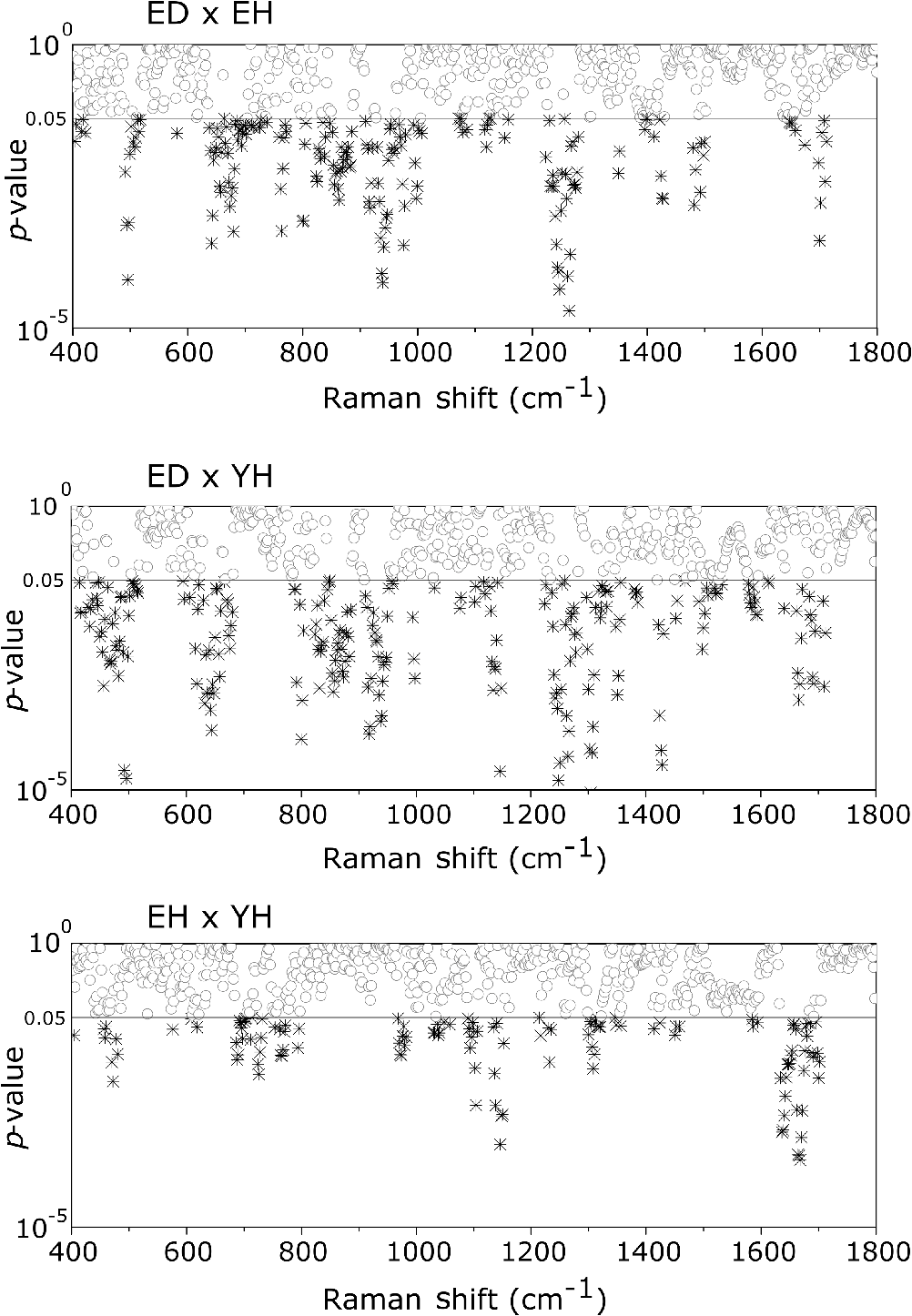 Figure 5 shows the results by univariate statistical approach for the three comparisons (ED versus EH, ED versus YH, and EH versus YH). Black stars represent the variables with statistically significant differences at 95% confidence level. Therefore, are represented by black stars and are represented by open circles. The region below the horizontal line () shows the candidates that can act as vibrational markers for each comparison. In order to be more specific, emphasis will be given to the spectral region between 800 and . This spectral region does not show any significant variables for comparing EH versus YH, but for comparing ED versus EH and ED versus YH, many variables appear as significant. In other words, the spectral region between 800 and appears to be a good spectral marker to differentiate the group of ED to other groups, but it does not show significant difference in the comparison between the YH and EH groups. The vibrational modes in this spectral region 800 to mainly correspond to the region of amino acids P and HP.34,35 The considerations for a multivariate statistical approach start from the right side of the flowchart shown in Fig. 4. In case of spectral overlap [see Fig. 3(a)] or in case of very difficult analysis by visual inspection or in case of the presence of many vibrational modes, multivariate analysis provides good results by use of dimension reduction techniques.19 With the advantage of visualization of the behavior of the samples using a much smaller number of dimensions than spectral variables, this multivariate analysis is also useful in quantifying compounds. In multivariate analysis, we will discuss two different approaches: unsupervised analysis by PCA and supervised analysis by PLS-DA. PCA is a method of dimension reduction, in which the new variables called principal components (PCs) are projected in hyperplanes in such a way that the dispersion between the original variables is maximum. This approach is extremely useful for the data whose matrices are in the order of tens to hundreds of columns and can therefore be visualized in diagrams in two or three dimensions. The multivariate approach for the full Raman spectra of 30 samples after preprocessing steps is described in Sec. 2. The PCA model was fitted with three PCs with coefficient of explained variation of data matrix . The diagram of score plot for this PCA model is shown in Fig. 6(a). The PCA diagram shows evidence of the formation of groups of samples, which reinforces the importance of the proposed study as the PCA analysis is based only on the spectra of the samples without any additional information, i.e., the samples are grouped in accordance with their confocal Raman spectra profile. However, the PCA model is influenced by individual characteristics such as age, skin pigmentation, and any other variable that was not controlled, thus presenting a very good way to inspect the experiment and detect outliers. It is not mandatory to use unsupervised methods such as PCA before a supervised analysis. However, this step is recommended to detect the outliers where there is no provision of any detailed information. Fig. 6Multivariate statistical analysis: (a) nonsupervised PCA analysis and (b) supervised PLS-DA analysis for young healthy (YH), elderly healthy (EH), and elderly with diabetes mellitus (ED) groups. 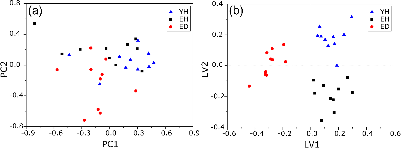 Figure 6(a) shows the position of the samples in the space of PCs. PCA is an unsupervised method that is extremely useful in detecting outliers and natural groupings based solely on the information of spectra. In this figure, it is possible to identify the tendency to form clusters; however, this does not occur due to intrinsic variability of each volunteer. When there is no clear separation among the groups in the PCA, score and loading plot analysis cannot be performed as it does not explain any group behavior. Since the goal of the study is to find characteristics of groups and not of individuals, supervised methods maximize the classification of samples owing to the characteristics of groups, reducing the effect of variables that contain the characteristics of individuals. A supervised model of PLS-DA was performed after the use of OSC on the sets of samples. For the PLS-DA approach, it is necessary to have some additional information along with the spectra of the sample like the origin of the samples or the group to which it belongs so that the algorithm tries to classify the samples into groups and consequently highlights the spectral regions responsible for their separation into groups. Figure 6(b) shows the PLS-adjusted model with and coefficient of variation explained of the discriminant class . In this model, the samples are grouped more efficiently than when compared with the PCA model, presenting complete separation of the groups. When this separation occurs, it is possible to ascertain which variables from the data matrix were uppermost, i.e., with higher weight for explaining the classification of the groups. These most important variables are then interpreted as the candidates for vibrational markers because they make the difference between these analyzed groups. As the PLS-DA model was more robust and showed good results to discriminate the three groups of samples, the subsequent strategy was to perform comparisons of two groups with the PLS-DA approach and then to check which spectral regions of confocal Raman spectra were the most important variables to explain this separation. With this approach, it is possible to verify the contribution of each original variable and wavenumber to explain the separation of the data into groups (Fig. 7). The graph as shown in Fig. 7 was performed using a variable extraction method of variable importance in the projection (VIP),45–47 where the higher the intensity of the peak, the greater the significance of that wavenumber in the separation of the groups. The list of VIP variables and the coefficient prediction capability , described in the Appendix, are obtained from rounds of cross-validation and have confidence intervals from Jack-knifing estimate. As the objective of this study is not to validate a new method, all other additional figures of merit that are generally used for various quantitative studies and comparisons with established techniques like limits of detection and quantification, root mean square, bias, sensibility and sensitivity, and curve ROC48–50 were not discussed in this article. Fig. 7Graph of VIP for PLS-DA model of young healthy (YH), elderly healthy (EH), and elderly with diabetes mellitus (ED).  The results obtained by univariate and multivariate analyses can be complementary. This is clearly observed from the comparison of the results of univariate and multivariate analyses as shown in Figs. 5 and 7, respectively. In the present study, as per the results of PLS-DA model, spectral region between 800 and on the graph appears to have important variables and this is the region that stands out most to explain the differences between ED and other groups in univariate analysis, thus corroborating and complementing the results obtained by univariate analysis. One of the goals of this study is to disseminate the knowledge on proper application of various statistical tools to the academic community. For this purpose, a complete routine of analysis including all the statistical tests used in this study is presented in the Appendix using the free R software. R software is a language and an environment for statistical computing, providing a wide variety of statistical and graphical techniques. It runs on a wide variety of platforms like UNIX, FreeBSD, Linux, Windows, and MacOS. 4.ConclusionsThis paper summarizes different statistical tools that can be implemented easily in spectroscopic techniques to reveal vibrational markers for the analysis of biological samples. Univariate approaches like parametric and nonparametric with all necessary assumptions required for the correct inference and evaluation of -values were dealt with in detail. In the case of the multivariate analysis, models of the PCA and PLS-DA were exemplified to find patterns in the sets of spectra, to detect outliers, and to suggest good candidates that act as vibrational markers. To evaluate the reproducibility and representativity of these measurements, the Pearson correlation matrix was applied. In addition to this, the HCA was used as an important tool for detecting outliers and grouping sets of measurements in confocal Raman spectroscopy. The application of these statistical tools was exemplified on confocal Raman dataset related to in vivo human skin analysis. The principal vibrational markers for skin aging using these statistical approaches were determined mainly in the spectral region between 800 and . This region is assigned for the amino acids P and HP, constituents of collagen responsible for skin framework and strength, and these amino acids are also associated with the formation of AGEs. For these reasons, P and HP are considered as potential biomarkers for explaining the chronological aging of skin and hyperglycemic effect on skin. This explanation was corroborated and complemented by these vibrational markers revealed in this study. To conclude, this work clearly emphasizes the need of vibrational markers for proper and speedy analysis of large sets of spectroscopic data. AppendicesAppendix:Routine of Data AnalysisIn this appendix, the suggested routine of data analysis for revealing vibrational markers in spectroscopic analysis is presented. This material includes various univariate tests like Kruskal–Wallis (nonparametric), Lilliefors (for normality), F-test (for variance), and -test. Multivariate approach comprises PCA and PLS-DA. Apart from these, HCA and Pearson correlation matrix were also included in this material. All lines of commands were performed by free R software. R software and additional packages necessary for this application are available as free downloads in the official page of R software. It is important to note that the statistical analysis is performed after the preprocessing of data. Therefore, spikes removal, baseline correction, smoothing, as well as data normalization that come under this preprocessing are not included in this discussion. #opening the data table data=read.table(file=“datatable.txt”, sep=“\t”,header=T, dec=“.”) #importing the data to R Software. Is crucial for statistical analysis the data will be imported correctly. dim(data) #verify the dimension of data, number of spectra (samples) in the lines and number of wavenumbers (variables) in the columns groupA=10 #enter the number of individuals in the control group groupB=10 #enter the number of individuals in the case group #Hierarquical Cluster Analysis - HCA library (hyperSpec) #package necessary spectra.dist=pearson.dist(alignment) #Pearson distance measure spectra.hclust=hclust(spectra.dist,method=“ward.D”) #Ward linkage method plot(spectra.hclust) #Dendrogram figure #Pearson correlation matrix #only for Pearson correlation matrix is necessary the transpose of data library (corrplot) #package necessary corrplot(cor(x, y, method = “pearson”), method = “number”) #Pearson matrix correlation figure #Univariate analysis class=c(rep(1, groupA),rep(2, groupB)) class=factor(class) variables=dim(data)[2] wavenumbers=c(data.frame(colnames(data))) #Calculation of -values for normality in each class with the Lilliefors test pvalLillieforsgroup1=rep(0,variables) pvalLillieforsgroup2=rep(0,variables) group1=data[class==1,] group2=data[class==2,] library(nortest) #package necessary for (i in 1:variables) {lillie1=lillie.test(group1[,i]) lillie2=lillie.test(group2[,i]) pvalLillieforsgroup1[i]=lillie1$p.value pvalLillieforsgroup2[i]=lillie2$p.value} #Calculation of -values for homogeneity of variances with the F-test pvalF=rep(0,variables) library(stats) #package necessary for (i in 1:variables) {testf=var.test(data[,i]∼class) pvalF[i]=testf$p.value} #Calculation of -values for t-test assuming different variances pvalTstudvardif=rep(0,variables) library(stats) #package necessary for (i in 1:variables) {tstudentvardif=t.test(data[,i]∼class) pvalTstudvardif[i]=tstudentvardif$p.value} # Calculation of -values for t-test assuming equal variances pvalTstudvarequal=rep(0,variables) library(stats) #package necessary for (i in 1:variables) {tstudentvarequal=t.test(data[,i]∼class,var.equal=TRUE) pvalTstudvarequal[i]=tstudentvarequal$p.value} #Calculation of -values for the nonparametric test of Kruskal-Wallis pvalkruskal=rep(0,variables) library(stats) #package necessary for (i in 1:variables) {kruskalwallis=kruskal.test(data[,i]∼class) pvalkruskal[i]=kruskalwallis$p.value} #Table with -values for all univariate statistical tests pvalues=data.frame(wavenumbers,pvalLillieforsgroup1,pvalLillieforsgroup2,pvalF,pvalTstudvardif,pvalTstudvarequal,pvalkruskal) write.table(pvalues, “univariatestatistics.csv”, sep=“,”, dec=“.”) #to save a table with all -values of the complete univariate analysis # Multivariate analysis #Principal component analysis - PCA pca.clase=c(rep(1, groupA),rep(2, groupB)) library(stats) #package necessary pcaanalysis=prcomp(data, scale. = TRUE, center = TRUE) #scaling and centering the data plot(summary(pcaanalysis)$importance[2,], ylab = “Proportion of variance”, xlab = “Number of PCs”) #Figure with Proportion of variance versus number of PCs plot(pcaanalysis$x, xlab = paste(“PC 1 (Proportion of Variance “, round(100*summary(pcaanalysis)$importance[2,1], dig = 2), “%)”, sep = ““), ylab = paste(“PC 2 (Proportion of Variance “, round(100*summary(pcaanalysis)$importance[2,2], dig = 2), “%)”, sep = ““), pch = pca.clase) #Figure with score plot of PCA summary(pcaanalysis) #summary of PCA coefficients #Partial least squares Discriminant analysis - PLS-DA plsda.clase=c(rep(1, groupA),rep(2, groupB)) library(DiscriMiner) #package necessary pls.analysis=plsDA(data, plsda.clase, autosel = TRUE) #scaling and centering the data plot(pls.analysis$components, xlab = paste(“PC 1; global (“, round(100*pls.analysis$R2[2,2], dig = 2), “%); global (“, round(100*pls.analysis$R2[2,4], dig = 2), “%); global (“, round(100*pls.analysis$Q2[1,3], dig = 2), “%)”, sep = ““), ylab = paste(“PC 2”), pch = plsda.clase) # Figure with score plot of PLS-DA summary(pls.analysis) #summary of PCA coefficients write.table(pls.analysis$VIP, “VIP-plsda.csv”, sep=“\t”, dec=“.”) #to save a table with the list of Variables importance in the projection (VIP) of the first latent variable. AcknowledgmentsAuthors thank FVE, CNPq, FINEP, and CAPES [Project Numbers 88881.062547/2014-01 (T. O. Mendes), 8887.068264/2014-00 (L. dos Santos), and 88881.068140/2014-01 (V. K. Tippavajhala)] for their financial support. A. A. Martin acknowledges CNPq (307809/2013-7). ReferencesR. S. Das and Y. K. Agrawal,
“Raman spectroscopy: recent advancements, techniques and applications,”
Vib. Spectrosc., 57
(2), 163
–176
(2011). http://dx.doi.org/10.1016/j.vibspec.2011.08.003 Google Scholar
D. Pappas, B. W. Smith and J. D. Winefordner,
“Raman spectroscopy in bioanalysis,”
Talanta, 51
(1), 131
–144
(2000). http://dx.doi.org/10.1016/S0039-9140(99)00254-4 TLNTA2 0039-9140 Google Scholar
S. Wachsmann-Hogiu, T. Weeks and T. Huser,
“Chemical analysis in vivo and in vitro by Raman spectroscopy—from single cells to humans,”
Curr. Opin. Biotechnol., 20
(1), 63
–73
(2009). http://dx.doi.org/10.1016/j.copbio.2009.02.006 Google Scholar
K. Virkler and I. K. Lednev,
“Raman spectroscopy offers great potential for the nondestructive confirmatory identification of body fluids,”
J. Forensic Sci., 181
(1–3), e1
–e5
(2008). http://dx.doi.org/10.1016/j.forsciint.2008.08.004 Google Scholar
L. Franzen and M. Windbergs,
“Applications of Raman spectroscopy in skin research—from skin physiology and diagnosis up to risk assessment and dermal drug delivery,”
Adv. Drug Delivery Rev., 89 91
–104
(2015). http://dx.doi.org/10.1016/j.addr.2015.04.002 ADDREP 0169-409X Google Scholar
J. R. Baena and B. Lendl,
“Raman spectroscopy in chemical bioanalysis,”
Curr. Opin. Biotechnol., 8
(5), 534
–539
(2004). http://dx.doi.org/10.1016/j.cbpa.2004.08.014 Google Scholar
R. Liu et al.,
“Applications of Raman-based techniques to on-site and in-vivo analysis,”
TrAC, Trends Anal. Chem., 30
(9), 1462
–1476
(2011). http://dx.doi.org/10.1016/j.trac.2011.06.011 TTAEDJ 0165-9936 Google Scholar
S. Wold, K. Esbensen and P. Geladi,
“Principal component analysis,”
Chemom. Intell. Lab. Syst., 2
(1–3), 37
–52
(1987). http://dx.doi.org/10.1016/0169-7439(87)80084-9 Google Scholar
I. T. Jolliffe, Principal Component Analysis, Springer, New York
(2002). Google Scholar
P. Geladi and B. R. Kowalski,
“Partial least-squares regression: a tutorial,”
Anal. Chim. Acta, 185 1
–17
(1986). http://dx.doi.org/10.1016/0003-2670(86)80028-9 ACACAM 0003-2670 Google Scholar
S. Wold, M. Sjöström and L. Eriksson,
“PLS-regression: a basic tool of chemometrics,”
Chemom. Intell. Lab. Syst., 58
(2), 109
–130
(2001). http://dx.doi.org/10.1016/S0169-7439(01)00155-1 Google Scholar
T. Fearn,
“On orthogonal signal correction,”
Chemom. Intell. Lab. Syst., 50
(1), 47
–52
(2000). http://dx.doi.org/10.1016/S0169-7439(99)00045-3 Google Scholar
S. Wold et al.,
“Orthogonal signal correction of near-infrared spectra,”
Chemom. Intell. Lab. Syst., 44
(1–2), 175
–185
(1998). http://dx.doi.org/10.1016/S0169-7439(98)00109-9 Google Scholar
J. Trygg and S. Wold,
“Orthogonal projections to latent structures (O-PLS),”
J. Chemom., 16
(3), 119
–128
(2002). http://dx.doi.org/10.1002/cem.695 Google Scholar
M. Barker and W. Rayens,
“Partial least squares for discrimination,”
J. Chemom., 17
(3), 166
–173
(2003). http://dx.doi.org/10.1002/cem.785 Google Scholar
M. Bylesjö et al.,
“OPLS discriminant analysis: combining the strengths of PLS-DA and SIMCA classification,”
J. Chemom., 20
(8–10), 341
–351
(2006). http://dx.doi.org/10.1002/cem.1006 Google Scholar
L. Kaufman and P. J. Rousseeuw, Finding Groups in Data: An Introduction to Cluster Analysis, 1
–67
(2008). http://dx.doi.org/10.1002/9780470316801.ch1 Google Scholar
M. Forina et al.,
“A new algorithm for seriation and its use in similarity dendrograms,”
Chemom. Intell. Lab. Syst., 87
(2), 262
–274
(2007). http://dx.doi.org/10.1016/j.chemolab.2007.03.004 Google Scholar
J. Moros, S. Garrigues and M. d. l. Guardia,
“Vibrational spectroscopy provides a green tool for multi-component analysis,”
TrAC, Trends Anal. Chem., 29
(7), 578
–591
(2010). http://dx.doi.org/10.1016/j.trac.2009.12.012 Google Scholar
C. Kendall et al.,
“Raman spectroscopy, a potential tool for the objective identification and classification of neoplasia in Barrett’s oesophagus,”
J. Pathol., 200
(5), 602
–609
(2003). http://dx.doi.org/10.1002/path.1376 Google Scholar
N. Stone et al.,
“Near-infrared Raman spectroscopy for the classification of epithelial pre-cancers and cancers,”
J. Raman Spectrosc., 33
(7), 564
–573
(2002). http://dx.doi.org/10.1002/jrs.882 JRSPAF 0377-0486 Google Scholar
C. Krafft et al.,
“Near infrared Raman spectroscopic mapping of native brain tissue and intracranial tumors,”
Analyst, 130
(7), 1070
–1077
(2005). http://dx.doi.org/10.1039/B419232J ANLYAG 0365-4885 Google Scholar
S. Fendel and B. Schrader,
“Investigation of skin and skin lesions by NIR-FT-Raman spectroscopy,”
Fresenius’ J. Anal. Chem., 360
(5), 609
–613
(1998). http://dx.doi.org/10.1007/s002160050767 Google Scholar
C. M. Krishna et al.,
“Micro-Raman spectroscopy of mixed cancer cell populations,”
Vib. Spectrosc., 38
(1–2), 95
–100
(2005). http://dx.doi.org/10.1016/j.vibspec.2005.02.018 Google Scholar
J. Filik and N. Stone,
“Analysis of human tear fluid by Raman spectroscopy,”
Anal. Chim. Acta, 616
(2), 177
–184
(2008). http://dx.doi.org/10.1016/j.aca.2008.04.036 Google Scholar
L. d. O. Nunes et al.,
“FT-Raman spectroscopy study for skin cancer diagnosis,”
Spectroscopy, 17
(2, 3), 597
–602
(2003). http://dx.doi.org/10.1155/2003/104696 Google Scholar
A. Molckovsky et al.,
“Diagnostic potential of near-infrared Raman spectroscopy in the colon: differentiating adenomatous from hyperplastic polyps,”
Gastrointest. Endosc., 57
(3), 396
–402
(2003). http://dx.doi.org/10.1067/mge.2003.105 Google Scholar
K. W. Short et al.,
“Raman spectroscopy detects biochemical changes due to proliferation in mammalian cell cultures,”
Biophys. J., 88
(6), 4274
–4288
(2005). http://dx.doi.org/10.1529/biophysj.103.038604 Google Scholar
P. Crow et al.,
“The use of Raman spectroscopy to identify and grade prostatic adenocarcinoma in vitro,”
Cancer Res., 89
(1), 106
–108
(2003). http://dx.doi.org/10.1038/sj.bjc.6601059 Google Scholar
M. R. Almeida et al.,
“Classification of Amazonian rosewood essential oil by Raman spectroscopy and PLS-DA with reliability estimation,”
Talanta, 117 305
–311
(2013). http://dx.doi.org/10.1016/j.talanta.2013.09.025 TLNTA2 0039-9140 Google Scholar
M. Muratore,
“Raman spectroscopy and partial least squares analysis in discrimination of peripheral cells affected by Huntington’s disease,”
Anal. Chim. Acta, 793 1
–10
(2013). http://dx.doi.org/10.1016/j.aca.2013.06.012 Google Scholar
R Core Team,
“R: A language and environment for statistical computing,”
Vienna, Austria
(2015). https://www.R-project.org/ Google Scholar
H. L. Royden and P. M. Fitzpatrick, Real Analysis, 4th ed.Prentice Hall, New York
(1988). Google Scholar
L. Pereira et al.,
“Confocal Raman spectroscopy as an optical sensor to detect advanced glycation end products of the skin dermis,”
Sens. Lett., 13
(9), 791
–801
(2015). http://dx.doi.org/10.1166/sl.2015.3523 Google Scholar
C. A. Téllez et al.,
“RM1 semi empirical and DFT: B3LYP/3-21G theoretical insights on the confocal Raman experimental observations in qualitative water content of the skin dermis of healthy young, healthy elderly and diabetic elderly women’s,”
Spectrochim. Acta, Part A, 149 1009
–1019
(2015). http://dx.doi.org/10.1016/j.saa.2015.06.110 Google Scholar
A. K. Palmer and J. L. Kirkland,
“Aging and adipose tissue: potential interventions for diabetes and regenerative medicine,”
Exp. Gerontol., S0531
(2016). http://dx.doi.org/10.1016/j.exger.2016.02.013 Google Scholar
S. Paliwal et al.,
“Diagnostic opportunities based on skin biomarkers,”
Eur. J. Pharm. Sci., 50
(5), 546
–556
(2013). http://dx.doi.org/10.1016/j.ejps.2012.10.009 EPSCED 0928-0987 Google Scholar
T. Bocklitz et al.,
“How to pre-process Raman spectra for reliable and stable models?,”
Anal. Chim. Acta, 704
(1–2), 47
–56
(2011). http://dx.doi.org/10.1016/j.aca.2011.06.043 ACACAM 0003-2670 Google Scholar
R. Gautam et al.,
“Review of multidimensional data processing approaches for Raman and infrared spectroscopy,”
EPJ Tech. Instrum., 2
(1), 1
–38
(2015). http://dx.doi.org/10.1140/epjti/s40485-015-0018-6 Google Scholar
P. Lasch,
“Spectral pre-processing for biomedical vibrational spectroscopy and microspectroscopic imaging,”
Chemom. Intell. Lab. Syst., 117 100
–114
(2012). http://dx.doi.org/10.1016/j.chemolab.2012.03.011 Google Scholar
C. C. Aggarwal and P. S. Yu,
“Outlier detection for high dimensional data,”
SIGMOD Rec., 30
(2), 37
–46
(2001). http://dx.doi.org/10.1145/376284.375668 Google Scholar
H. W. Lilliefors,
“On the Kolmogorov-Smirnov test for normality with mean and variance unknown,”
J. Am. Stat. Assoc., 62
(318), 399
–402
(1967). http://dx.doi.org/10.1080/01621459.1967.10482916 Google Scholar
M. Hollander, D. A. Wolfe and E. Chicken, Nonparametric Statistical Methods, John Wiley & Sons, Inc., Hoboken, New Jersey
(1999). Google Scholar
G. W. Snedecor and W. G. Cochran, Statistical Methods, 8th ed.Iowa State University Press, Ames, Iowa
(1989). Google Scholar
N. L. Afanador, T. N. Tran and L. M. C. Buydens,
“Use of the bootstrap and permutation methods for a more robust variable importance in the projection metric for partial least squares regression,”
Anal. Chim. Acta, 768 49
–56
(2013). http://dx.doi.org/10.1016/j.aca.2013.01.004 ACACAM 0003-2670 Google Scholar
I.-G. Chong and C.-H. Jun,
“Performance of some variable selection methods when multicollinearity is present,”
Chemom. Intell. Lab. Syst., 78
(1–2), 103
–112
(2005). http://dx.doi.org/10.1016/j.chemolab.2004.12.011 Google Scholar
T. Mehmood et al.,
“A review of variable selection methods in partial least squares regression,”
Chemom. Intell. Lab. Syst., 118 62
–69
(2012). http://dx.doi.org/10.1016/j.chemolab.2012.07.010 Google Scholar
T. Fawcett,
“ROC graphs: notes and practical considerations for data mining researchers,”
Palo Alto, California
(2003). Google Scholar
G. D. Doddridge and Z. Shi,
“Multivariate figures of merit (FOM) investigation on the effect of instrument parameters on a Fourier transform-near infrared spectroscopy (FT-NIRS) based content uniformity method on core tablets,”
J. Pharm. Biomed. Anal., 102 535
–543
(2015). http://dx.doi.org/10.1016/j.jpba.2014.10.019 Google Scholar
C. Beleites, R. Salzer and V. Sergo,
“Validation of soft classification models using partial class memberships: an extended concept of sensitivity & co. applied to grading of astrocytoma tissues,”
Chemom. Intell. Lab. Syst., 122 12
–22
(2013). http://dx.doi.org/10.1016/j.chemolab.2012.12.003 Google Scholar
BiographyThiago de Oliveira Mendes received his bachelor’s, master’s, and PhD degrees in physics from Federal University of Juiz de Fora, Brazil. As a PhD student, he worked with vibrational spectroscopy applied to food and drug analysis, especially in the development of protocols for multicomponent quantification. Currently, he is pursuing his postdoctoral fellowship under the supervision of Dr. Airton Abrahao Martin in the analysis of different types of biological samples by confocal Raman and infrared spectroscopy. Liliane Pereira Pinto received her bachelor’s degree from the University of Alfenas, Brazil, and her master’s degree in biomedical engineering from the Universidade do Vale do Paraíba, Brazil. She is currently working with vibrational spectroscopy applied to skin aging and glycation analysis for her PhD in biomedical engineering from Universidade do Vale do Paraiba, Brazil. Laurita dos Santos received her MSc and PhD degrees in applied computing from National Institute for Space Research (INPE), Brazil, in 2009 and 2013, respectively. She is currently pursuing her postdoctoral fellowship in biomedical engineering from Universidade do Vale do Paraiba, São José dos Campos, Brazil. Vamshi Krishna Tippavajhala received his bachelor’s and master’s degrees in pharmacy from Kakatiya University, India. He worked on “Multiparticulate drug delivery systems for Tuberculosis therapy” during his PhD in Manipal University, India. Currently, he is working on “Confocal Raman spectroscopic analysis of cosmetic permeation through human skin” for his postdoctoral fellowship under the guidance of Prof. Airton Abrahao Martin in the Laboratory of Biomedical Vibrational Spectroscopy, Universidade do Vale do Paraiba, Brazil. Claudio Alberto Téllez Soto is a full professor in inorganic chemistry from the UFF University, Brazil (retired). Currently, he is working as a scientific researcher in the Institute of Research and Development (IP&D), University of Vale do Paraíba (UNIVAP), Brazil. His research area is vibrational spectroscopy applied to all the chemistry branches, medicine, odontology, and biological sciences. He has guided 20 master’s degree and 12 PhD students and authored more than 100 papers. Airton Abrahão Martin received his bachelor’s, master’s, and PhD degrees in physics from State University of Londrina in 1985, University of São Paulo in 1988, and University of Toronto and Unicamp in 1995, respectively. He did his postdoctorate at Max Planck Institute for Festokoperforschung—Stuttgart in 1999. He also holds an MSc degree from the University of Toronto, Canada, in 1991. Currently, he is an associate professor, coordinator of the Biomedical Engineering Graduate program, and head of LEVB, UNIVAP, Brazil. |