
|
|
1.IntroductionNear-infrared spectroscopy (NIRS) is one of the widely used noninvasive techniques for monitoring brain function assay and breast imaging. It makes use of the optical properties such as absorption and scattering to provide the pathophysiological information about the tissue under investigation. The wavelength window between 650 and 950 nm, also known as the NIR window, is often utilized for NIR imaging due to less absorption and scattering of light in biological tissues. The NIR light that propagates in the tissue goes under multiple scatterings; modeling of this NIR light propagation in the tissue has been an active area. Moreover, these models provide insights into the clinical/experimental investigations that are either carried out or being planned. These models are often repetitively utilized in NIR image reconstruction procedures and are extremely useful to assess the sensitivity/specificity of the experimental investigations.1–4 Light propagation under multiple scattering conditions, which is typically the case for tissues having thickness , has been modeled accurately either using radiative transfer equation (RTE) or Monte Carlo (MC) simulation. In case of thin tissues, the Beer–Lambert law is often utilized, but its utility is often limited, especially for in vivo imaging cases. The modified Beer–Lambert law (MBLL) is an empirical description of light propagation in thick tissues, widely used in NIRS.5–7 This utilizes a “differential pathlength factor” (DPF), which gives a ratio of the mean photon pathlength to the source detector distance. The DPF values are usually taken from the literature for a given tissue type and often require additional measurements (time-resolved ones) to accurately estimate these values.8 Note also that DPF values are dependent on the source–detector distance and require a careful choice for obtaining useful information. There have been various studies to show that this model may be applicable for measuring global changes in the optical absorption coefficient and incapable of determining the relative local (focal) changes in it.9 However, in the past,10–12 there have been investigations on the accuracy of MBLL. Boas et al.10 observed that the results of optical simulation for in vivo data suggested that standard MBLL analysis cannot accurately quantify relative changes in the concentration of chromophores. In fact, standard MBLL analysis could produce inaccurate results due to uncontrolled changes in DPF with the source–detector positions and optical properties of the medium. Uludag et al.12 also observed the erroneous calculation due to the partial volume effect and its wavelength dependence. The RTE, which is an accurate model for light propagation in biological tissues, can be further simplified by representing the solution in the form of spherical harmonics, which leads to an system of connected partial differential equations known as the approximation. These could be further reduced to a single differential equation of order (). For , it leads to the popular diffusion equation (DE). The MBLL is based on RTE solution’s functional dependence on .13 The limitation of RTE usage in modeling the light propagation in biological tissues lies with the computational complexity, which often requires very lengthy computer run times. The DE is relatively efficient compared to RTE, but has limitations in terms of its validity for all tissue types. It is applicable when the absorption coefficient of tissue is much less than its reduced scattering coefficient (i.e., ) and the light goes under multiple scattering (thickness ).14 The MC simulation provides a numerical model for random migration of photons in tissue and known to be a gold standard for modeling NIR light propagation. It is universally applicable for all tissue types and tissue length scales. In this, NIR light is modeled as distinct photon packets, which are traced through the tissue with utilization of random numbers and optical properties of tissue.15 To achieve reasonable accuracy, the MC simulation requires a large number of photon packets to be traced through the tissue due to the statistical nature of modeling. It becomes prohibitively expensive in terms of computation time when the absorption coefficient is much less than the scattering coefficient as the photon packet may propagate a long distance before being exited/absorbed in the tissue. In lieu of existing modeling methods for light propagation in biological tissue, there is a clear niche for an improved model, which is universally applicable and overcomes the limitations of existing models. Here, we introduce Lambert-W function-based modeling, which is a generalized version of the well-known Beer–Lambert law. The Lambert-W function has applications in various scientific disciplines, and recently it has been utilized in modeling of kilovoltage x-ray beam attenuation.16 It will be shown that the proposed model has a computational complexity far less compared with the existing methods and provides a close match to the gold standard modeling techniques, such as MC simulation. Moreover, this also provides an easy and intuitive parameterization of tissue optical properties based on Lambert-W function. In the end, a comprehensive discussion of how this parameterization correlates with optical absorption and scattering coefficients was also provided. Note that, as the discussion here is limited light attenuation in the biological tissue, the comparison of applicability of the proposed model was performed with pure-intensity (attenuation) data. 2.Methods2.1.Modified Beer–Lambert LawAs mentioned earlier, the MBLL is widely used in NIR spectroscopic data analysis to quantify the changes in tissue chromophore concentrations. DPF is a parameter that accounts for increases in photon pathlength due to multiple light scattering in tissue.1,17–19 The theory of MBLL has been explained earlier in Refs. 5 and 6. Briefly, it provides an empirical model for description of optical attenuation in highly scattering medium. The MBLL is given by or alternatively where is the detected light intensity, is the incident light intensity, OD is the optical density, is the source–detector distance, and is the optical absorption coefficient. log is a natural algorithm with base . and are appropriate factors that account for the measurement geometry. The total mean path length of detected photons is . Recently, Sassaroli and Fantini6 showed that the above equation is partially incorrect. should be written as its average over the range of the absorption coefficient , i.e.,The term represents the mean average path length. If can be regarded constant and the absorption changes homogeneously in the illuminated tissue volume; then, for relatively small changes of attenuation, Eq. (2) leads to the definition of DPF as Note that in this work, the measurement geometry has been identical in all the experiments carried out, essentially making not having any effect on the comparison of presented results. Further, while considering two OD data points for interpolation purpose, i.e., (), cancels out. Thus, making the factor ineffective. Given Eq. (4), now DPF can be related to tissue optical properties, namely optical absorption coefficient () and reduced scattering coefficient () by using the diffusion theory. 2.1.1.Infinite geometry model solutionThe equation of steady-state photon diffusion in a homogeneous medium is where is the photon density, is the diffusion coefficient, and is the source term. This equation has a well-known closed-form solution of the form20 where . By using the definition of DPF provided by Fantini et al.21 or Arridge et al.,22 for an infinite geometry model, diffusion theory gives the following relationship between DPF and the optical parameters of the tissue21,232.1.2.Semi-infinite geometry model solutionSimilar to the above analysis, for the semi-infinite geometry, the formula between DPF and optical coefficients can be given as23–26 However, DPF for semi-infinite geometry increases with the increase in source–detector distance and reaches an asymptotic value.21 Note that both of these DPF definitions for these geometries are obtained by utilizing Green’s function solution to DE in these geometries. Obviously, and semi-infinite geometry is widely used for noninvasive diffuse wave reflectance spectroscopy. As these analytical definitions have shown to have a good agreement with experimentally found values, we also utilized these formulas for the MBLL model. It is to be noted that the DPF formula given by Eq. (8) depends upon the source–detector distance, while the other Eq. (7) does not. Although semi-infinite geometry is widely preferred in NIRS experiments, the infinite geometry solution provides a quick way of calculating the optical properties without having dependency on the source–detector distance. This [formula given by Eq. (7)] provides a powerful tool to analyze NIRS data. 2.2.Monte Carlo ModelThe MC model provides a numerical, rather statistical, solution of RTE and is used as the gold standard for describing light propagation in tissue. The MC model is widely applicable irrespective of the tissue thickness, optical properties, and source–detector distance. It is described in detail in Refs. 14 and 27. Briefly, a photon packet with an initial weight of unity is launched in orthogonal direction to the tissue surface. Then, a step size is chosen based on a random number with the help of the following expression: where is a random number equidistributed between 0 and 1, is the optical scattering coefficient, and is the step size. At each step, the photon packet is split into two parts; one part is absorbed and another transmitted (scattered). The fraction that is transmitted is given by where is the weight of the scattered (transmitted) photon after each interaction and is the original weight before interaction. The scattered photon direction is computed by the Henyey–Greenstein phase function, which gives the deflection angle as where is called as the anistropic factor; note that . The azimuthal angle is also distributed over the interval 0 to and is sampled asThe interaction of the photon packet with the tissue surface is modeled with the help of Fresnel’s equation, primarily to determine the internal reflection. The photon is terminated when the weight of the photon is less than a preset threshold (here, ). Often, a “Russian roulette” is used to a give a chance to the terminable photon packet. If the photon packet exits in the boundary of the tissue, then the photon packet weight is contributed to the diffuse reflectance or transmittance. If reflection occurs, the photon packet is again traced until it exits or terminates. Afterward, another photon packet is launched into the medium. This process is repeated until statistically meaningful results are obtained, usually requiring about 1 to 10 million photon packets to be launched. In this work, 100 million photon packets are traced as the source–detector distance was in the range of 3 to 40 mm, as well as to obtain higher signal-to-noise ratio values for the diffuse reflectance/transmittance measurements. To keep the computational run times lower, the parallel implementation of MC simulation was utilized as described in Ref. 15. 2.3.Diffusion EquationFor most biological tissues in the NIR spectral range, the reduced scattering coefficient () is much larger than the absorption coefficient (). As the discussion in this work is about thick biological tissues, which tend to be highly diffusive, the DE provides a good model for describing the light propagation in tissues. The DE is given by where and represent the isotropic light source and diffuse photon density/intensity (real values), respectively, at position and is the diffusion coefficient. In a space invariant medium, this equation becomes as Eq. (5). is found by solving this partial differential equation [Eq. (13)] using finite-element method (FEM), providing versatility in accommodating irregular geometries.28–30 We have utilized the near infrared fluorescence and spectral tomography (NIRFAST) package,31 which is based on the FEM formulation and data type being diffuse transmittance/ reflectance.2.4.Generalized Beer–Lambert Law (Proposed Model)The MBLL describes the attenuation of photons as they propagate along a medium and is described by Eq. (1). Many analytical models have been proposed to improve the accuracy of photon attenuation models in higher energy side of the light spectrum.32–34 As mentioned earlier, a recently proposed empirical model was proven to be more accurate for narrow poly-energetic x-ray beam, which effectively took into account the scattering of x-ray photons. Similar to that, we propose a parameterization for describing the attenuation of NIR light through biological tissue as which is a standard Beer–Lambert’s law, but here, is written as where and are two unknown parameters that represent the optical properties in the proposed parameterization scheme. Substituting Eqs. (15) in (14) results inRearranging terms leads to which is of the Lambert-W function (also known as omega function, represented by ) form. That is of the form Equating Eqs. (17) and (18) makes whose solution involves the Lamber-W function (readers are advised to refer to Appendix A of16) given byNote that is a multivalued inverse of the function defined in Eq. (18). Also, when and , it reduces to Eq. (1) (MBLL). Therefore, Eq. (20) represents a generalized form of the Beer–Lambert law. In this case, OD can be written as The two attenuation coefficients and are included in the generalized Beer–Lambert law (GBLL). These are not an alternative to DPF, which is used to compute the more accurate path length. They provide a way of parametrization to describe NIR light propagation in biological tissues. 2.5.Physical Significance of andFrom Eqs. (15) and (20), the proposed model can be written as The rate of change of total attenuation coefficient, i.e., can be written as So, the rate of change of (total attenuation coefficient) varies with distance . The larger the distance from the NIR light source is, the smaller the variation in is.For the case , the value of Lambert-W function is 0.35 The derivative of W function with respect to is . The value of the derivative at , i.e., . This converts Eq. (22) as follows: and as tends to infinite boundary, where all photons gets attenuated, this becomesThe total attenuation coefficient at distance , half value layer, quarter value layer, and at infinity is listed in Table 1, Table 1Total attenuation coefficients versus distance/depth x.
This analysis infers the following:
Thus, the two parameters and can be defined as follows. is the attenuation coefficient at which light would have attenuated per unit length in the absence of scattering events. is the finite change in total attenuation coefficient () as the light travels from the tissue surface to the infinite boundary, within a turbid media, like biological tissue. This means is going to be the minimum value of the total attenuation coefficient that the incident NIR photon beam will ever go through. The nearest detectors from the source will observe larger total attenuation coefficient (). The decrease in will happen gradually and reach a minimum at infinite source–detector separation. 2.6.Normalization of the DataThe intensity values can be computed from Eq. (20). However, these values are very small and range up to 10th to 12th exponents in decimals. To avoid the round-off error, we consider OD, a similar quantity computed in logarithmic domain. The OD is given by Eq. (21), which is derived from Eq. (20). The normalization has been performed to lower the dynamic range of OD and for easy interpretation of results. The OD data was divided with the first OD value (at the first suitable detector), in -line with normalizations performed in the literature. This normalization also takes care of variations in the source modeling, including the source strength. Note that, in our experience, the normalization of experimental data to reduce the dynamic range helps to find the optimal parameters ( and ) that provide the least-squares fit. Then, the model values are rescaled to map the original dynamic range. Equation (21) was fit to OD versus source–detector distance () data in MATLAB R2013b by nonlinear least square regression, which used the Levenberg–Marquardt algorithm36 to determine the values of the two parameters and . The and values for various tissues have been mentioned in Table 4. This table also explores the relation between these two parameters and the diffusion coefficient . 3.Numerical ExperimentsMC simulations (parallel implementation by Qiang15) were performed to assess the parameters and of the proposed model and compare the various light propagation models discussed here. A semi-infinite mesh with a depth of 2.5 cm (-axis) and another mimicking infinite media (the depth being ) were considered for numerical experiments for semi-infinite and infinite geometry, respectively. These two geometries were utilized in MBLL computations, as the DPF value is different for the two types of geometries. As required in MC simulations,15 the grid element was fixed at in size. The anisotropy factor of the tissues was considered as , and the refractive index was kept as . The first detector was placed at 0.1-cm distance from the irradiating laser source, and the consecutive next detectors were placed at 0.2-cm distance apart from one another in a straight line, as shown in Fig. 1. The tissue layers were surrounded with air on both sides and had the optical properties as described in Table 2. A schematic diagram of source and detector placement is shown in Fig. 1. Fig. 1The placement of detectors as kept in numerical experiments carried out for MC simulations. is the laser source and are the detectors.  Table 2Optical properties of various biological soft tissues.
Simulation data for a total of 10 biological tissues are considered in this study. The MC simulation was carried with one million photons, and the output of the simulation provided the reflectance values at these detectors. The study also utilized the NIRFAST package29 to obtain the diffusion model solution. 3.1.Choice of Lambert-W BranchThe Lambert-W function is defined as the multivalued inverse of the function . This function is also known as the omega function or the product log function. is the omega constant and can be considered a “golden ratio” of exponents. The Lambert-W function has many applications in pure and applied mathematics.35 Since it is a multivalued function, it has many branches on real and complex planes. The zeroth branch, also called the principal branch, is the special branch as it can contain the whole of the positive real axis in its range. The detailed description of the branches and applications of the Lambert-W function is beyond the scope of this study; the detailed explanation can be found in Ref. 35. Note that in many physical applications, including modeling of kilovoltage x-ray beam attenuation,16 only the principal branch was utilized. For completeness, we compared the zeroth, first, and second branch modeling against the MC model and investigated the best fit within these branches. 3.2.Validation of Generalized Beer–Lambert LawThe proposed study represents a GBLL to model the absorption in NIRS. These numerical experiments validate the proposed Beer–Lambert model by comparing it with the traditional MC15 and NIRFAST31 simulation models. Beyond the 1-cm source–detector separation, the proposed model provides an accurate model for describing NIR light propagation in thick tissues. However, this study observes that the proposed Beer–Lambert model does not match well for the nearest tissues where the source–detector distance , which is due to the dominating Mie scattering events occurring at the smaller thickness.37 As discussed earlier, there are two geometries that are typically used in NIR spectroscopic experiments, one is the infinite turbid medium geometry and other is the semi-infinite geometry. We also included these two models that are present in the literature38 in our validation studies. Note that as these infinite and semi-infinite geometries are approximations to the tissue geometries; the obtained OD values are normalized to have the same initial value as with MC model in all results presented in this work. 3.3.Biological Tissues Considered in this WorkThe optical characteristics of the soft tissues, i.e., the absorption coefficient and the scattering coefficient, are the important parameters for the study. We have validated the proposed model’s robustness for various biological tissues. The optical properties of the tissues that are utilized in the investigations performed are listed in Table 2.14,21,39–46 4.ResultsInitially, we compare the proposed Beer–Lambert model with the simulated MC reflectance data. The purpose of the study is to validate it for biological tissues. Hence for a general soft tissue, we have chosen the absorption coefficient as and the scattering coefficient as . The proposed generalized Beer–Lambert model is compared to existing MBLL and the MC model to observe the accuracy of the proposed model. 4.1.Validation of Proposed Model for Biological TissuesWe validate the proposed model by plotting the absorption values versus source–detector distance and comparing them with the previously established models. The results for a general biological tissue with the given optical properties are shown in Figs. 2 and 3. For the nearest detectors ( source detector distance), Fig. 2(a) shows that the validation does not hold well. However, beyond the 1-cm distance, both the plots are close; Fig. 2(b) implies that the proposed model fits well at relevant distances from source location. The same validation is also performed with the NIRFAST modulation for an in-built simple circular geometry (which is different than the geometry used for generating Fig. 2). Figure 3 shows the validation of the proposed model compared with the DE-based numerical model data for the distance . Fig. 2Comparison of proposed generalized Beer–Lambert’s model against MC simulation for source–detector distances (a) and (b) .  Fig. 3Comparison of proposed generalized Beer–Lambert’s model against diffusion model (NIRFAST simulation) for source–detector distances . 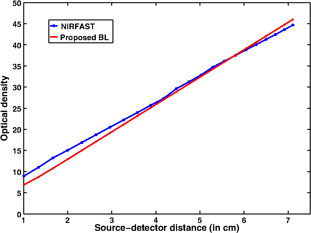 At smaller source–detector separations [, refer to Fig. 2(a)], the model does not hold well due to the presence of Mie scattering events. The first truthful point, which gives correct OD value, is beyond1 cm. The Lambert-W function was plotted for the various branches of (zeroth, first, and second branch) against the MC model in Fig. 4. The zeroth branch makes the obvious choice, as the first and second branches are far away from the MC data. Fig. 4Comparison of various Lambert-W branches to justify the choice of zeroth branch as the best fit for the proposed generalized Beer–Lambert’s model against MC simulation.  To better validate our proposed model, three types of human tissues were considered: gray matter, scalp and skull, and breast tissue. Figures 5 and 6 shows the absorption value plots for these three types of the tissues and for the each of the models discussed here, in semi-infinite and infinite geometry, respectively. It is clear from these two figures that the proposed model validates well with the MC data compared with MBLL, which is existent in the literature. Fig. 5Proposed generalized Beer–Lambert model, MC simulation, and MBLL plots of source–detector distance versus OD for semi-infinite turbid medium [Eq. (8)] for human tissues: (a) gray matter, (b) scalp and skull, and (c) breast.  Fig. 6Proposed generalized Beer–Lambert model, MC simulation, and MBLL plots of source–detector distance versus OD for infinite turbid medium [Eq. (7)] for human tissues: (a) gray matter, (b) scalp and skull, and (c) breast.  The same study is also performed for the animal tissues. The optical properties for the animal tissues are listed in Table 2. Figure 7 shows the absorption value plots for rat muscle and piglet head, in semi-infinite and infinite geometry, respectively. The observed trend is similar to human tissues, thus validating that the proposed generalized Beer–Lambert model holds well for both human and animal tissue types. Fig. 7Proposed generalized Beer–Lambert model, MC simulation, and MBLL plots of source–detector distance versus OD for (a) semi-infinite turbid medium, rat muscle; (b) semi-infinite turbid medium, piglet head; (c) infinite turbid medium, rat muscle; and (d) infinite turbid medium, piglet head.  The most prominent application of NIRS is to study the human brain function.47,48 Keeping this in mind, we validated our model for an inhomogeneous tissue model for human brain. We prepared a tissue model with four layers of scalp and skull, gray matter, CSF, and white matter. The layers widths were kept as 1, 1, 0.5, and 0.5 cm, respectively. The results are shown in Fig. 8(a). The optical properties of layers are mentioned in Table 340,41 The MC simulation output closely matches with the proposed model. More importantly, even in low-scattering tissue cases49 like synovial membrane as shown in Fig. 8(b), the proposed model closely follows the MC results, implying that the proposed model can be used even in low-scattering tissue cases. Table 3Optical properties of different layers of the inhomogeneous tissue at 630 nm.
Fig. 8Proposed generalized Beer–Lambert model against MC simulation for (a) an inhomogeneous tissue comprising of layers (adult head model) with the optical properties as defined in Table 3 and (b) synovial membrane (low-scattering tissue). 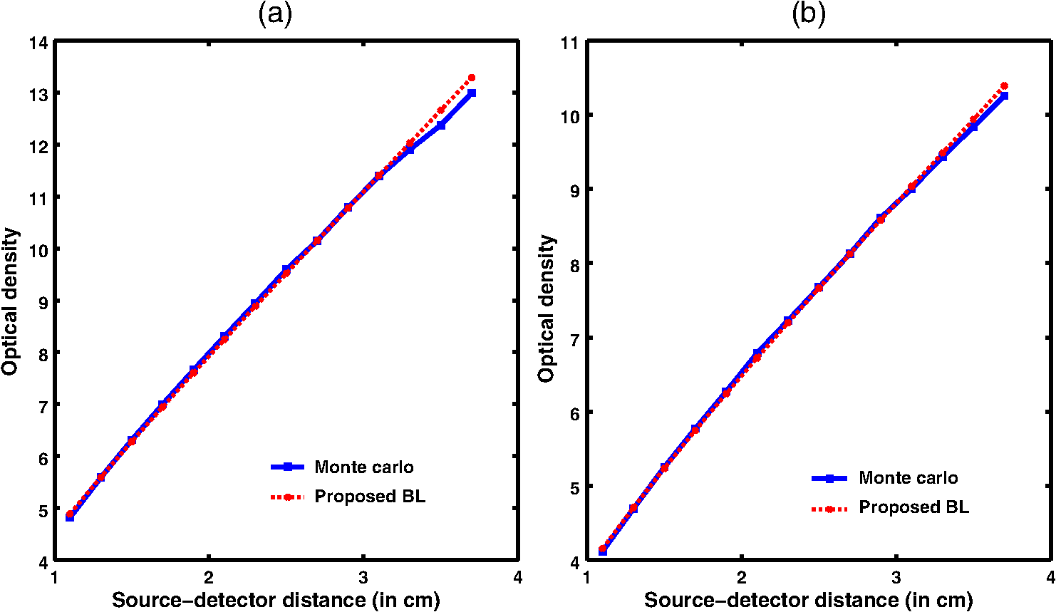 4.2.Validation for Nondiffusive TissueOne of the major approximation for diffusion model to be valid is . Table 2 lists the optical properties of the various biological tissues. It must be observed that most biological tissues come under the diffusion model approximation in NIR window. The aim of this investigation is to show that the proposed model is valid where the photon diffusion theory is valid. However, to show that the proposed model also works in the conditions where the photon diffusion model does not, we need to look at a tissue where is not true. The rat muscle tissues have this optical property at 980-mm wavelength,45 as listed in Table 2. The study solved the diffusion model (NIRFAST) as well as the MC and the proposed model for rat muscle tissue. The comparisons, shown in Fig. 9, make it explicit that the proposed model is valid where the photon diffusion model fails. 4.3.Parameters of Proposed Model: andThe proposed generalized Beer–Lambert model contains two parameters and . Our study observes that the parameter has a direct relationship with the effective absorption coefficient, i.e., with . We found that is proportional to this value and increases with the same slope. Table 4 lists the comparison of these parameters. It is also observed that constantly decreases with , i.e., they are in inverse proportion. We plotted two curves versus and versus to justify the relation (Fig. 10), asserting that the proposed model is in close agreement with the known literature. The future work includes a detailed investigation of the parameters and and their relation with the tissue optical properties. Table 4List of the optical parameters of various soft biological tissues. μ0 and η are the parameters discussed in the proposed model [Eq. (16)]. The list clearly shows that μ0 and η has a direct relationship with (3μaμs′) for both human tissues and animal tissues.
Fig. 10Comparison of the two parameters and of the proposed model with the effective absorption coefficient, a function of absorption coefficient, and scattering coefficient. This figure was plotted for different biological tissues. While has a linearly decreasing characteristic, follows an increasing pattern as the function varies.  5.DiscussionThis study proposed a generalized Beer–Lambert model for light propagation in thick tissues, using the Lambert-W function. The experiments conducted here showed that the proposed model accurately describes the photon attenuation in biological tissues for source–detector distances . In this work, both human and animal tissue types were considered to demonstrate the versatility of the model. Furthermore, we also considered inhomogeneous and low-scattering tissues to assert that the proposed model has universal applicability across tissue types. The accurate model for light propagation in biological tissues uses RTE, with its equivalent statistical model being the MC simulation. However, these models are computationally expensive. Therefore, the focus of this study was on developing a universal model that overcomes the limitation of existing models. The proposed Lambert-W function-based Beer–Lambert model closely models the photon attenuation in biological tissues, in the NIR spectral range, where multiple scattering and even low-scattering tissue cases were incorporated. The accuracy of the proposed generalized Beer–Lambert model is very promising compared to MBLL, which uses DPF to model the light propagation. DPF depends on the optical properties of the tissue. DPF also changes initially with source–detector distance and then becomes stable. This makes the standard MBLL analysis produce inaccurate results.10 Moreover, the proposed model provides parameterization for modeling the NIR light propagation in biological tissue above 1 cm thickness. The promising results may motivate future development in understanding the role of parameterization that is provided in this work ( and ), as they have been proposed in the kilovoltage x-ray beams.16 The results presented in this work indicated that the proposed model may not fit well at very small distances between source and detectors (less than 1 cm). This is mainly attributed to, at smaller source detector separations, scattering following Mie theory calculations and is a more complicated function of , with enhanced sensitivity of elastic scatter measurements at smaller separations.37 Disagreement in reflectance values between the experimental and theoretical models at small source–detector separations were also found in the past in a diffuse light propagation study.37,50 The previous semi-infinite geometry model used by Fantini et al.,21 solved the DE and used the DPF scheme. Our study compared the results with these models. It was found that the MC data, which is considered to be a gold standard, deviated substantially with the MBLL model. However, the proposed model overcame this limitation and matched well with the MC data. We also validated our model for rat muscle tissue (Fig. 9), where DE is not valid due to being extremely low (i.e., not true). The correlation of the optical absorption coefficient and scattering coefficient with and was also considered in this study. The developed model parameters follow a linear trend with the effective absorption coefficient (Fig. 10). The future scope of the study is to establish the and more accurately and develop an inverse model to accurately determine these in phantom as well as patient cases. For fair comparison, the average computational time for the proposed model for a general biological tissue(with and ) is 3.3 s as compared to MC simulation taking 54 s on a Windows workstation with Intel Quadcore processor (2.4 GHz) having 8 GB memory. 6.ConclusionThe generalized Beer–Lambert model proposed in this study describes the light propagation in thick biological tissues. The developed model has a distinct advantage of its universal applicability on par with the MC model for tissue thicknesses beyond 1 cm. Applications of the proposed model in NIRS include brain and breast imaging. The advantage of using Lambert-W function-based modeling is that it is less computationally expensive, making it very appealing in both dynamic as well as video-rate NIRS studies. AcknowledgmentsThe authors would like to thank Dr. Sree Ram Valluri (University of Western Ontario) for the initial discussions on this work. This work was supported by the Department of Biotechnology (DBT) Innovative Young Biotechnologist Award (IYBA) (Grant No. BT/07/IYBA/2013-13), the Department of Biotechnology (DBT) Rapid Grant for Young investigator (RGYI) (No: BT/PR6494/GDB/27/415/2012), and DBT Bioengineering (Grant No. BT/PR7994/ MED/32/284/2013). The work of M.B. was supported by the National Mathematics Initiative (NMI). ReferencesA. D. Edwards et al.,
“Measurement of hemoglobin flow and blood flow by near-infrared spectroscopy,”
J. Appl. Physiol., 75
(4), 1884
–1889
(1993). Google Scholar
M. Cope and D.T. Delpy,
“System for long-term measurement of cerebral blood flow and tissue oxygenation on newborn infants by infra-red transillumination,”
Med. Biol. Eng. Comput., 26
(3), 289
–294
(1988). http://dx.doi.org/10.1007/BF02447083 MBECDY 0140-0118 Google Scholar
M. Cope,
“The development of a near-infrared spectroscopy system and its application for noninvasive monitoring of cerebral blood and tissue oxygenation in the newborn infant,”
Univ. College London,
(1991). Google Scholar
T. H. Foster et al.,
“Oxygen consumption and diffusion effects in photodynamic therapy,”
Radiat. Res., 126
(3), 296
–303
(1991). http://dx.doi.org/10.2307/3577919 RAREAE 0033-7587 Google Scholar
L. Kocsis, P. Herman and A. Eke,
“The modified Beer–Lambert law revisited,”
Phys. Med. Biol., 51
(5), N91
–N98
(2006). http://dx.doi.org/10.1088/0031-9155/51/5/N02 PHMBA7 0031-9155 Google Scholar
A. Sassaroli and S. Fantini,
“Comment on the modified Beer–Lambert law for scattering media,”
Phys. Med. Biol., 49
(14), N255
–N257
(2006). http://dx.doi.org/10.1088/0031-9155/49/14/N07 PHMBA7 0031-9155 Google Scholar
W. B. baker et al.,
“Modified Beer–Lambert law for blood flow,”
Biomed. Opt. Express, 5
(11), 4053
–4075
(2014). http://dx.doi.org/10.1364/BOE.5.004053 BOEICL 2156-7085 Google Scholar
G. Strangman, M. A. Franceschini and D. A. Boas,
“Factors affecting the accuracy of nearinfrared spectroscopy concentration calculations for focal changes in oxygenation parameters,”
NeuroImage, 18
(4), 865
–879
(2003). http://dx.doi.org/10.1016/S1053-8119(03)00021-1 NEIMEF 1053-8119 Google Scholar
T. Durduran,
“Non-invasive measurements of tissue hemodynamics with hybrid diffuse optical methods,”
University of Pennsylvania,
(2004). Google Scholar
D. A. Boas et al.,
“The accuracy of near infrared spectroscopy and imaging during focal changes in cerebral hemodynamics,”
NeuroImage, 13
(1), 76
–90
(2001). http://dx.doi.org/10.1006/nimg.2000.0674 NEIMEF 1053-8119 Google Scholar
T. J. Germon et al.,
“Cerebral near infrared spectroscopy: emitter-detector separation must be increased,”
Br. J. Anaesthesia, 82
(6), 831
–837
(1999). http://dx.doi.org/10.1093/bja/82.6.831 BJANAD 0007-0912 Google Scholar
K. Uludag et al.,
“Cross talk in the Lambert-Beer calculation for near-infrared wavelengths estimated by Monte Carlo simulations,”
J. Biomed. Opt., 7
(1), 51
–59
(2002). http://dx.doi.org/10.1117/1.1427048 JBOPFO 1083-3668 Google Scholar
J. J. Duderstadt and W. R. Martin, Transport Theory, Wiley, New York
(1979). Google Scholar
V. Tuchin, Tissue Optics: Light Scattering Methods and Instruments for Medical Diagnosis, SPIE Press, Bellingham, Washington
(2010). Google Scholar
B. Qiang, J. Ni and L. L. Fajardo,
“Parallel Monte Carlo algorithm for simulation of photon migration inside biological tissues,”
in 93rd RSNA Scientific Assembly and Annual Meeting,
25
–30
(2007). Google Scholar
K. B. Mathieu et al.,
“An empirical model of diagnostic X-ray attenuation under narrow-beam geometry,”
Med. Phys., 38
(8), 4546
–4555
(2011). http://dx.doi.org/10.1118/1.3592933 MPHYA6 0094-2405 Google Scholar
J. H. Meek et al.,
“Regional changes in cerebral haemodynamics as a result of a visual stimulus measured by near infrared spectroscopy,”
Proc. R. Soc. B Biol. Sci., 261
(1362), 351
–356
(1995). http://dx.doi.org/10.1098/rspb.1995.0158 PRLBA4 0080-4649 Google Scholar
M. Cope et al.,
“Data analysis methods for near infrared spectroscopy of tissues: problems in determining the relative cytochrome aa3 concentration,”
Proc. SPIE, 1431 251
–263
(1991). http://dx.doi.org/10.1117/12.44196 PSISDG 0277-786X Google Scholar
M. R. Stankovic et al.,
“Optical monitoring of cerebral hemodynamics and oxygenation in the neonatal piglet,”
J. Matern. Fetal Invest., 8
(2), 71
–78
(1998). Google Scholar
A. Zhang et al.,
“Photon diffusion in a homogeneous medium bounded externally or internally by an infinitely long circular cylindrical applicator. I. Steady-state theory,”
J. Opt. Soc. Am. A, 27
(3), 648
–662
(2010). http://dx.doi.org/10.1364/JOSAA.27.000648 JOAOD6 0740-3232 Google Scholar
S. Fantini et al.,
“Non invasive optical monitoring of the newborn piglet brain using continuos-wave and frequency-domain spectroscopy,”
Phys. Med. Biol., 44
(6), 1543
–1563
(1999). http://dx.doi.org/10.1088/0031-9155/44/6/308 PHMBA7 0031-9155 Google Scholar
S. R. Arridge, M. Cope and D. T. Delpy,
“The theoretical basis for the determination of optical pathlengths in tissue: temporal and frequency analysis,”
Phys. Med. Biol., 37
(7), 1531
–1560
(1992). http://dx.doi.org/10.1088/0031-9155/37/7/005 PHMBA7 0031-9155 Google Scholar
D. Piao et al.,
“On the geometry dependence of differential pathlength factor for near-infrared spectroscopy. I. Steady-state with homogeneous medium,”
J. Biomed. Opt., 20
(10), 105005
(2015). http://dx.doi.org/10.1117/1.JBO.20.10.105005 JBOPFO 1083-3668 Google Scholar
H. Liu et al.,
“Simplified approach to characterize optical properties and blood oxygenation in tissue using continuous near infrared light,”
496
–502
(1995). http://dx.doi.org/10.1117/12.209998 Google Scholar
T. J. Farrel, M. S. Patterson and B. Wilson,
“A diffusion theory model of spatially resolved, steady-state diffuse reflectance for the noninvasive determination of tissue optical properties in vivo,”
Med. Phys., 19
(4), 879
–888
(1992). http://dx.doi.org/10.1118/1.596777 MPHYA6 0094-2405 Google Scholar
M. S. Patterson, B. Chance and B. C. Wilson,
“Time resolved reflectance and transmittance for the non-invasive measurement of optical properties,”
Appl. Opt., 28
(12), 2331
–2336
(1989). http://dx.doi.org/10.1364/AO.28.002331 APOPAI 0003-6935 Google Scholar
S. T. Flock, B. C. Wilson and M. S. Patterson,
“Hybrid Monte Carlo-diffusion theory modeling of light distributions in tissue,”
20
–28
(1988). http://dx.doi.org/10.1117/12.945337 Google Scholar
S. R. Arridge and M. Schweiger,
“Photon-measurement density functions. Part 2: Finite-element-method calculations,”
Appl. Opt., 34
(34), 8026
–8037
(1995). http://dx.doi.org/10.1364/AO.34.008026 APOPAI 0003-6935 Google Scholar
H. Dehghani et al.,
“Numerical modelling and image reconstruction in diffuse optical tomography,”
Phil. Trans. R. Soc. A Math. Phys. Eng. Sci., 367
(1900), 3073
–3093
(2009). http://dx.doi.org/10.1098/rsta.2009.0090 PTRMAD 1364-503X Google Scholar
M. Schweiger et al.,
“The finite element model for the propagation of light in scattering media: boundary and source conditions,”
Med. Phys., 22
(11), 1779
–1792
(1995). http://dx.doi.org/10.1118/1.597634 MPHYA6 0094-2405 Google Scholar
H. Dehghani et al.,
“Near infrared optical tomography using NIRFAST: algorithms for numerical model and image reconstruction algorithms,”
Commun. Numer. Methods Eng., 25
(6), 711
–732
(2009). http://dx.doi.org/10.1002/cnm.v25:6 CANMER 0748-8025 Google Scholar
C. Kleinschmidt,
“Analytical considerations of beam hardening in medical accelerator photon spectra,”
Med. Phys., 26
(9), 1995
–1999
(1999). http://dx.doi.org/10.1118/1.598704 Google Scholar
B. E. Bjarngard and H. Shackford,
“Attenuation in high-energy x-ray beams,”
Med. Phys., 21
(7), 1069
–1073
(1994). http://dx.doi.org/10.1118/1.597349 Google Scholar
M. K. Yu, R. S. Sloboda and B. Murray,
“Linear accelerator photon beam quality at off-axis points,”
Med. Phys., 24
(2), 233
–239
(1997). http://dx.doi.org/10.1118/1.598069 Google Scholar
R. M. Corless, G. H. Gonnet, D. E. G. Hare, D. J. Jeffrey and D. E. Knuth,
“On the Lambert W function,”
Adv. Comput. Math., 5
(1), 329
–359
(1996). http://dx.doi.org/10.1007/BF02124750 ACMHEX 1019-7168 Google Scholar
D. W. Marquardt,
“An algorithm for least-squares estimation of nonlinear parameters,”
J. Soc. Ind. Appl. Math., 11
(2), 431
–441
(1963). http://dx.doi.org/10.1137/0111030 JSIMAV 0368-4245 Google Scholar
J. R. Mourant et al.,
“Predictions and measurements of scattering and absorption over broad wavelength ranges in tissue phantoms,”
Appl. Opt., 36
(4), 949
–957
(1997). http://dx.doi.org/10.1364/AO.36.000949 APOPAI 0003-6935 Google Scholar
S. Fantini, M. A. Franceschini and E. Gratton,
“Semi-infinite-geometry boundary problem for light migration in highly scattering media: a frequency-domain study in the diffusion approximation,”
J. Opt. Soc. Am. B, 11
(10), 2128
–2138
(1994). http://dx.doi.org/10.1364/JOSAB.11.002128 JOBPDE 0740-3224 Google Scholar
R. Cubeddu et al.,
“In vivo Absorption and scattering spectra of human tissues in red and near infrared,”
Advances in Optical Imaging and Photon Migration, 21 Optical Society of America(1998). Google Scholar
A. Custo et al.,
“Effective scattering coefficient of the cerebral spinal fluid in adult head models for diffuse optical imaging,”
Appl. Opt., 45
(19), 4747
–4755
(2006). http://dx.doi.org/10.1364/AO.45.004747 APOPAI 0003-6935 Google Scholar
A. N. Yaroslavsky et al.,
“Optical properties of selected native and coagulated human brain tissues in vitro in the visible and near infrared spectral range,”
Phys. Med. Biol., 47
(12), 2059
–2073
(2002). http://dx.doi.org/10.1088/0031-9155/47/12/305 PHMBA7 0031-9155 Google Scholar
S. J. Matcher, M. Cope and D. T. Delpy,
“In vivo measurements of the wavelength dependence of tissue scattering coefficients between 760 and 900 nm measured with time resolved spectroscopy,”
Appl. Opt., 36
(1), 386
–396
(1997). http://dx.doi.org/10.1364/AO.36.000386 APOPAI 0003-6935 Google Scholar
M. Essenpreis et al.,
“Spectral dependence of temporal point spread functions in human tissues,”
Appl. Opt., 32
(4), 418
–425
(1993). http://dx.doi.org/10.1364/AO.32.000418 APOPAI 0003-6935 Google Scholar
H. Suzuki et al.,
“Simultaneous determination of absorption coefficients for skin and muscle tissues using spatially resolved measurements,”
Adv. Mater. Res., 222 309
–312
(2011). http://dx.doi.org/10.4028/www.scientific.net/AMR.222 ADMRBX 0568-0018 Google Scholar
W. Jiang et al.,
“Optical properties of biological tissues measured at infrared wavelengths,”
Biomedical Optics 2014, Optical Society of America(2014). Google Scholar
S. L. Jacques,
“Optical properties of biological tissues: a review,”
Phys. Med. Biol., 58
(11), R37
–R61
(2013). http://dx.doi.org/10.1088/0031-9155/58/11/R37 PHMBA7 0031-9155 Google Scholar
E. Okada and D. T. Delpy,
“Near-infrared light propagation in an adult head model. II. Effect of superficial tissue thickness on the sensitivity of the near-infrared spectroscopy signal,”
Appl. Opt., 42
(16), 2915
–2921
(2003). http://dx.doi.org/10.1364/AO.42.002915 APOPAI 0003-6935 Google Scholar
J. Steinbrink et al.,
“Determining changes in NIR absorption using a layered model of the human head,”
Phys. Med. Biol., 46
(3), 879
–896
(2001). http://dx.doi.org/10.1088/0031-9155/46/3/320 PHMBA7 0031-9155 Google Scholar
Y. P. Kumar and R. M. Vasu,
“Reconstruction of optical properties of low-scattering tissue using derivative estimated through perturbation Monte-Carlo method,”
J. Biomed. Opt., 9
(5), 1002
–1012
(2004). http://dx.doi.org/10.1117/1.1778733 JBOPFO 1083-3668 Google Scholar
A. Kienle et al.,
“Spatially resolved absolute diffuse reflectance measurements for noninvasive determination of the optical scattering and absorption coefficients of biological tissue,”
Appl. Opt., 35
(13), 2304
–2313
(1996). http://dx.doi.org/10.1364/AO.35.002304 APOPAI 0003-6935 Google Scholar
BiographyManish Bhatt received his BTech degree from the National Institute of Technology, Hamirpur, Himachal Pradesh, India, in 2011. Currently, he is a graduate student at the National Mathematics Initiative, Indian Institute of Science, Bangalore, India. Kalyan R. Ayyalasomayajula received his MSc (Engg) degree from the Indian Institute of Science, Bangalore, India. Currently, he is working toward his PhD at the Department of Information Technology, Uppsala University, Sweden. Phaneendra K. Yalavarthy received his MSc degree in engineering from the Indian Institute of Science (IISc), Bangalore, India, and his PhD in biomedical computation from Dartmouth College, Hanover, New Hampshire, in 2007. He is an associate professor at the Department of Computational and Data Sciences, IISc. His research interests include medical image computing, medical image analysis, and biomedical optics. |


