Focusing light through biological tissue and tissue-mimicking phantoms up to 9.6 cm in thickness with digital optical phase conjugation

Yuecheng Shen; Yan Liu; Cheng Ma; Lihong V. Wang

doi:10.1117/1.JBO.21.8.085001

12 August 2016 Focusing light through biological tissue and tissue-mimicking phantoms up to 9.6 cm in thickness with digital optical phase conjugation

Yuecheng Shen, Yan Liu, Cheng Ma, Lihong V. Wang

Author Affiliations +

Journal of Biomedical Optics, Vol. 21, Issue 8, 085001 (August 2016). https://doi.org/10.1117/1.JBO.21.8.085001

Abstract

Optical phase conjugation (OPC)-based wavefront shaping techniques focus light through or within scattering media, which is critically important for deep-tissue optical imaging, manipulation, and therapy. However, to date, the sample thickness in OPC experiments has been limited to only a few millimeters. Here, by using a laser with a long coherence length and an optimized digital OPC system that can safely deliver more light power, we focused 532-nm light through tissue-mimicking phantoms up to 9.6 cm thick, as well as through ex vivo chicken breast tissue up to 2.5 cm thick. Our results demonstrate that OPC can be achieved even when photons have experienced on average 1000 scattering events. The demonstrated penetration of nearly 10 cm (∼100 transport mean free paths) has never been achieved before by any optical focusing technique, and it shows the promise of OPC for deep-tissue noninvasive optical imaging, manipulation, and therapy.

1. Introduction

Focusing light through or inside scattering media is critical in many applications, such as high-resolution fluorescence imaging, noninvasive optogenetics, photodynamic/photothermal therapy, laser surgery, and optical tweezers. However, light scattering caused by the microscopic refractive index inhomogeneities inherent in biological tissue prohibits optical focusing beyond $\sim 1 mm$ in depth.¹^–³ To break this optical diffusion limit, various wavefront shaping approaches, including stepwise wavefront shaping,⁴ transmission matrix measurement,⁵ and optical phase conjugation (OPC),⁶ have been developed to focus light deep inside or through scattering media. However, the thicknesses of samples used in previous studies were limited to only a few millimeters or several transport mean free paths ( $l_{t}^{'}$ ), which is still relatively shallow for many preclinical and clinical applications. For example, the thickest biological tissue used in stepwise wavefront shaping was 5-mm-thick chicken breast tissue.⁷ In an analog OPC experiment based on a photorefractive crystal, 7-mm-thick chicken breast tissue ⁸ was used. Recently, 4-mm-thick chicken breast tissue was used in a digital OPC experiment based on an electronic camera and spatial light modulators (SLMs).⁹ Although the principle of wavefront shaping does not impose an upper bound on the number of scattering events that can be tolerated, practical considerations such as an insufficiently strong light signal, a short speckle correlation time, and an inadequate laser coherence length can restrict the thickness of the sample through which light can be focused.

Compared with the other two wavefront shaping approaches, OPC-based techniques determine the optimum wavefront globally based on time reversal, without the need to optimize for each degree of freedom in sequence. Thus, they achieve the shortest average mode time (the average operation time per degree of freedom¹⁰), which makes them more suitable for in vivo applications. Various OPC-based techniques have been demonstrated to focus light through or inside scattering media.⁶^,⁸^–²⁴ Figure 1 shows a typical OPC experiment. In part (a), a narrow incident beam is scattered and broadened by a scattering medium. The distorted wave coming out of the medium is intercepted by a phase conjugate mirror (PCM) that performs OPC. In part (b), the PCM produces the phase conjugate of the intercepted light in part (a). Based on time-reversal symmetry, the phase conjugated light retraces the original path back through the scattering medium and recovers the narrow incident beam. Compared with analog OPC, digital OPC (DOPC) achieves a much higher fluence reflectivity, hence is able to deliver more energy to the focus. Here, using a laser with a long coherence length and an optimized DOPC system that can safely deliver more light power, we demonstrate focusing 532-nm light through ex vivo chicken breast tissue up to 2.5 cm thick and through tissue-mimicking phantoms up to 9.6 cm thick. Although multiple-centimeter depth has been reached by imaging modalities such as ultrasound-modulated optical tomography²⁵ and photoacoustic imaging,²⁶ the nearly 10 cm ( $\sim 100 l_{t}^{'}$ ) penetration has never been achieved before by any optical focusing technique.

Fig. 1

Illustration of OPC. (a) A narrow beam illuminates a scattering medium and is scattered inside the medium. The distorted wave coming out of the medium is intercepted by a PCM. (b) The PCM generates phase conjugated light, which retraces the original path back through the scattering medium and recovers the narrow incident beam.

2. Method

A schematic of the DOPC setup is shown in Fig. 2. A continuous-wave laser (Verdi V10, Coherent) with a coherence length longer than 100 m was used as the light source. A long coherence length is desired because OPC relies on constructive interference among different optical paths. Since the optical path-length difference is proportional to the square of the thickness of the scattering medium (as derived in Appendix A), the required coherence length increases quadratically with the thickness of the medium.

Fig. 2

Schematic of the digital OPC system. AOM, acousto-optic modulator; BB, beam block; BS, beamsplitter; CL, camera lens; HWP, half-wave plate; L, lens; M, mirror; MLS, motorized linear stage; P, polarizer; PBS, polarizing beamsplitter; R, reference beam; S, sample beam; sCMOS, scientific CMOS camera; SLM, spatial light modulator.

2.1.

Wavefront Recording

The incident light was split into a reference beam (R) and a sample beam (S) by a polarizing beamsplitter (PBS), PBS2, with the splitting ratio controlled by a half-wave plate (HWP), HWP2. Two acousto-optic modulators shifted the frequency of R and S by 50 MHz and $50 MHz + 12 Hz$ , respectively. Thus, a beat with a frequency of $f_{b} = 12 Hz$ was generated between R and S. Then a lens pair composed of L3 and L4 expanded the beam diameter of R to 25 mm, which is able to cover the entire surface of a SLM (Pluto NIR II, Holoeye). For S, a mirror (M), M4, mounted on a motorized linear stage (MLS) was initially moved out of the light path to position 1 (see Fig. 2), and a lens pair composed of L5 and L6 expanded the beam diameter of S to 34 mm. Because tissue damage is determined by the light intensity on the sample surface, a broad incident beam can safely deliver much more light power than a narrow beam, thus enhancing the signal-to-noise ratio (SNR) of wavefront measurement. In principle, to efficiently deliver power, there is an optimum illuminating beam size dependent on the property of each sample.²⁷ In practice, we chose a beam size that was reasonably good for most samples we tested. The collecting lens L8, which was used in all previous OPC setups to collect the scattered light, was removed in our setup to avoid focusing the reading beam onto the tissue surface in the playback step, which might otherwise cause tissue damage. After passing through the sample, S was combined with R using a 50/50 beamsplitter (BS), BS2. Their interference pattern on the SLM was imaged onto a scientific CMOS camera (sCMOS), sCMOS1 (Pco.edge 5.5, PCO-TECH), by a camera lens with a magnification of 1:1.23. To measure the phase map of S using heterodyne holography¹⁵^,²⁸ (see Appendix B for details), the camera took four successive measurements $I_{1}$ , $I_{2}$ , $I_{3}$ , and $I_{4}$ at a frame rate of four times the beat frequency $f_{b} (= 48 Hz)$ . Based on these four measurements, the phase map of the sample beam $ϕ_{S} (x, y)$ was calculated by $ϕ_{S} (x, y) = Arg [(I_{1} - I_{3}) + i (I_{4} - I_{2})]$ , where $Arg [\cdot]$ computes the principal value of the argument of a complex number. To make our technique applicable to future in vivo applications that need to accommodate the fast speckle decorrelation of living tissue (on a time scale of milliseconds²³), the camera exposure time was set to 1 ms in all our experiments, and no averaging was used.

2.2.

Wavefront Reconstruction

To achieve OPC, in the playback step, the SLM displayed the conjugation of the measured phase map. In addition, S was blocked, and M4 was moved to position 2. After reflection from the SLM, R was phase modulated and became the phase conjugated light S*. Passing through the sample again, S* became collimated, reflected by M4, and focused by lens L7 onto sCMOS2. To compensate for the aberrations in the wavefront of R and the substrate curvature of the SLM, we digitally added orthogonal rectangular polynomials²⁹ to the SLM display, using the calibration method described in Ref. 30. It is estimated that the entire process, starting from the beginning of the wavefront measurement to the appearance of the focus on sCMOS2, took around 0.7 s (system runtime).

3. Result

3.1.

Focusing Light Through Chicken Breast Tissue

We demonstrate focusing light through chicken breast tissue in Fig. 3. The side views of two chicken samples with 2.5 and 2.0 cm thicknesses are shown in Fig. 3(a). The effective areas in the left and right surfaces for light input and output were $7.2 cm \times 7.2 cm$ , and all the other areas were masked with black aluminum foil tapes (T205-2.0, Thorlabs) to make sure that all the detected light had passed through the full thickness of the sample. All the experiments were performed within 2 days after sample preparation. The light intensity on the chicken tissue surface was $200 mW / {cm}^{2}$ , which is the same as the American National Standards Institute (ANSI) safety limit. Figure 3(b) shows images of the OPC foci after light passed through tissue samples with thicknesses ranging from 0.5 to 3.0 cm. With increasing sample thickness, the speckles in the background become more and more pronounced relative to the peak intensity of the focus. When the sample was 3.0 cm thick, no focus was observed. We quantified the contrast of the focus by the peak-to-background ratio (PBR), defined as the ratio between the average intensities within and outside the focal spot (whose size is defined by the full width at half maximum). Figure 3(c) shows that the PBR decreases with increasing sample thickness. Theoretically, the PBR for phase-only OPC can be calculated by $π N / (4 M)$ , where $N$ is the number of optical modes intercepted by the SLM and $M$ is the number of optical modes in the conjugated focus.²² Since $N / M$ was kept roughly the same during our experiments, the PBRs should, in theory, be a constant independent of the sample thickness.

Fig. 3

(a) Side view of two chicken breast tissue samples with 2.5 and 2.0 cm thicknesses. A cubic beamsplitter with a side length of 2.0 cm is also shown for comparison. (b) Images of the OPC foci after light has passed through chicken breast tissue of various thicknesses. (c) PBR as a function of sample thickness. The error bar shows the standard deviation obtained from three samples of the same thickness.

To explain the observed PBR drop, we examined two possibilities. The first probability is an insufficient SNR during wavefront measurement. Since the light power transmitted through the sample decreases exponentially with increasing sample thickness (see Appendix B, Fig. 7), when the transmitted light is too weak, errors in the measured phase map may become too large, which reduces the PBR. However, by using the numerical approach described in Appendix B, we found that even for the 2.5-cm thick sample, the reduction of PBR due to phase errors was only around 10%. Therefore, the PBR drop is not primarily due to an insufficient SNR. The second possibility is a faster speckle decorrelation rate with increasing sample thickness. The thicker the sample, the more scattering events the photons experience, and thus the shorter the speckle correlation time is.³¹ In theory, the speckle correlation time is inversely proportional to the square of the sample thickness.³² In our experiments, for samples thicker than 1.0 cm, the speckle correlation times were shorter than the system runtime. That is to say, the wavefront changed rapidly with time, and the measured wavefront was different from the correct one at the moment of playback. In this case, the PBR reduces to $η \times$ PBRc, where PBRc is the PBR achieved by using the correct wavefront, and $η$ is the PBR reduction coefficient, which, in the noise-free case, is determined by the absolute square of the correlation coefficient between the measured wavefront and the correct wavefront at the moment of playback.²¹ The fast speckle decorrelation for ex vivo chicken tissue is due to both the intrinsic and the laser-heating induced Brownian motion of scatterers. We note that although the SNR is not the primary factor that causes the PBR drop for the 2.5-cm-thick chicken sample, it can become the dominant factor for samples thicker than 3.7 cm. It is shown in Appendix B that in the decorrelation-free case, the PBR reduction coefficient $η$ starts to drop exponentially when the SNR becomes smaller than 1 ( $SNR = 1$ when $thickness = 3.7 cm$ ). For 5.0- and 6.0-cm thick samples, $η$ drops to 0.017 and 0.0012, respectively, showing that insufficient SNR can significantly degrade the performance of DOPC.

3.2.

Focusing Light Through Tissue-Mimicking Phantoms

Since red blood cells in biological tissue absorb green light strongly, 532 nm is not an optimal wavelength for thick tissue.³³ To reduce the light absorption by the sample, we switched to widely used tissue-mimicking intralipid-gelatin phantoms.³⁴ These phantoms have an absorption coefficient of $0.07 {cm}^{- 1}$ at 532 nm, which is close to that of chicken tissue at 800 nm ( $0.08 {cm}^{- 1}$ ), but their reduced scattering coefficient at 532 nm is larger than that of chicken tissue at 800 nm ( $10 {cm}^{- 1}$ versus $3.5 {cm}^{- 1}$ ).³³ Their scattering anisotropy $g$ is 0.9. Compared with chicken tissue, the phantoms are more mechanically stable. Figure 4(a) shows two phantoms with thicknesses of 9.6 and 8.5 cm, along with a forearm of a 28-year-old male adult. It can be seen that our samples are even thicker than the human arm. In our experiments, the light intensity on the phantom surface was $1.2 W / {cm}^{2}$ , six times as high as the ANSI safety limit. However, no damage was observed in the sample after the experiment. It is worth noting that the ANSI safety limit is usually more than 10 times below the observed damage threshold. Figure 4(b) shows images of the OPC foci after light has passed through phantoms with thicknesses ranging from 0.8 to 10.0 cm. We could focus light through a sample even with a thickness of 9.6 cm, although no focus was observed when the thickness was 10.0 cm. Focusing light through a 9.6-cm thick sample by DOPC is quite remarkable because the transmitted photons have experienced on average at least 1000 scattering events, and moreover, only a tiny portion of the entire scattered wavefront is phase conjugated (The collected light power was only $10^{- 9}$ of the incident power on the sample). Figure 4(c) shows the PBR as a function of sample thickness. When the thickness is no greater than 5.5 cm, the values of PBRs are very similar ( $\sim 170$ ). For thicker samples, the PBR drops with increasing thickness, because the speckle correlation time becomes shorter than the system runtime for these samples. Since the transmitted light power for the 9.6-cm-thick phantom is 23 times stronger than that for the 2.5-cm-thick chicken sample, insufficient SNR is not a major factor that causes the PBR drop.

Fig. 4

(a) Side view of the intralipid-galetin phantoms with 9.6 cm and 8.5 cm thicknesses. A forearm of a 28-year-old male adult is also shown for comparison. (b) Images of the OPC foci after light has passed through phantoms of various thicknesses. (c) PBR as a function of sample thickness. The error bar shows the standard deviation obtained from three samples of the same thickness.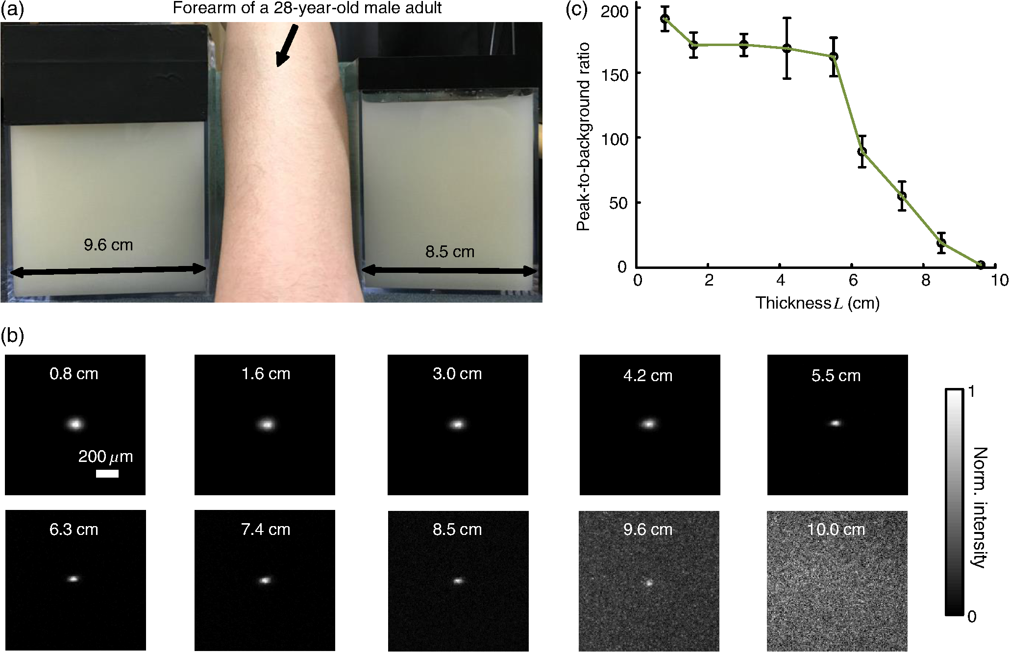

4. Discussion and Conclusion

Finally, we discuss the limitations of our study and potential improvements to the DOPC system. First, the fast speckle decorrelation of thick samples is the major factor that prohibits us from focusing light through thicker samples. To reduce the system runtime, we can use a faster MLS, and further optimize the data processing code. We may also use a digital micromirror device as a fast SLM, and employ single-shot phase measurement to speed up the wavefront measurement.²²^,²⁴ Second, we note that $π N / (4 M)$ describes the PBR in which the background intensity is calculated from the average intensity within the focal spot after ensemble averaging over many illuminating wavefronts. However, when applying optical focusing in real applications, the ratio between the average intensities within and outside the focal spot is more relevant and useful, and we define this ratio as the PBR. In our definition of the PBR, the background intensity is calculated from the average intensity outside the focal spot when the incident wavefront is optimal, and it is higher than the background intensity ensemble averaged over many illuminating wavefronts (in our case it is 10 times higher).³⁵ Thus, the measured PBR is smaller than $π N / (4 M)$ . For example, for a 0.8-cm-thick phantom, $π N / (4 M) \sim 9.0 \times 10^{4}$ , while the measured PBR is only around 200. The misalignment of the system also makes the measured PBR smaller than $π N / (4 M)$ . Third, assuming that we have a perfectly aligned system and extremely stable samples, the ultimate limit on the thickness of the sample that we can focus light through by OPC is determined by the SNR in the wavefront measurement (see Appendix B).³⁶ Therefore, when the SNR is limited by shot noise rather than a laser’s technical noise, it is desirable to have a strong laser that delivers as much light as possible while keeping the intensity on the sample surface under the safety limit.

In conclusion, using an optimized DOPC system, we focused 532-nm light through chicken tissue up to 2.5 cm thick and through tissue-mimicking phantoms up to 9.6 cm thick. The 9.6 cm ( $\sim 100 l_{t}^{'}$ ) penetration has never been achieved before by any optical focusing technique, and it shows the promise of OPC-based wavefront shaping techniques to revolutionize biomedicine with deep-tissue noninvasive optical imaging, manipulation, and therapy.

Appendices

Appendix A:

Requirement of Laser Coherence Length in OPC Experiments

Since focusing light through or inside scattering media by OPC relies on constructive interference of light that has propagated through different optical paths inside a scattering medium, a long laser coherence length is required. Ideally, the laser coherence length should be longer than the optical path-length difference among the various paths. Here, we develop an analytical model to estimate the path-length difference in a scattering medium. Based on the diffusion theory for an infinite medium, under a first-order approximation, a pencil beam illuminating a scattering medium can be modeled as an isotropic source located one transport mean free path (1 $l_{t}^{'}$ ) beneath the sample surface³^,³⁷ [see Fig. 5(a)]. At time $t$ , the laser fluence rate at a distance $r$ from the isotropic point source can be calculated by³

Eq. (1)

φ (r, t > r / c) = \frac{c}{{(4 π D c t)}^{3 / 2}} \exp (- \frac{r^{2}}{4 D c t} - μ_{a} c t),

where

c

is the speed of light in the scattering medium and

D

is the diffusion coefficient.

D = 1 / [3 (μ_{a} + μ_{s}^{'})]

, where

μ_{a}

and

μ_{s}^{'}

are the absorption coefficient and the reduced scattering coefficient of the scattering medium. The point source is placed at the origin of the coordinate system. For mathematical convenience, we first assume that

μ_{a}

is zero. The effect of a nonzero

μ_{a}

on the path-length difference will be discussed at the end of this section. At a given location

r

, Fig. 5(b) shows the normalized

φ (r, t)

with respect to the time delay

t

. By setting the partial derivative with respect to

t

to zero, we find that the time delay for the maximum fluence rate is

t_{\max} = r^{2} / 6 D c

. That is to say, photons are most likely to spend time

t_{\max}

to reach position

r

. In order to allow photons to interfere efficiently at position

r

, the laser coherence time should at least reach the full width at half maximum (FWHM) of the distribution. By multiplying the coherence time with

c

, the minimum laser coherence length is obtained.

Fig. 5

(a) Schematic of photon paths to reach the location denoted by the red dot in a scattering medium. (b) Normalized photon fluence rate as a function of time delay $t$ at a given position $r$ .

To determine the two moments $t_{left}$ and $t_{right}$ when the normalized fluence rate drops to 0.5, based on Eq. (1) and $t_{\max} = r^{2} / 6 D c$ , we write

Eq. (2)

\frac{φ}{φ (t_{\max})} = {(\frac{t_{\max}}{t})}^{3 / 2} \exp (- \frac{r^{2}}{4 D c t}) \exp (\frac{3}{2}) = \frac{1}{2},

which can be rewritten as

Eq. (3)

{(\frac{1}{t})}^{3 / 2} \exp (- \frac{r^{2}}{4 D c t}) = \frac{1}{2} {(\frac{1}{e t_{\max}})}^{3 / 2} .

For equations in the format of

{(1 / t)}^{3 / 2} \exp (- a / t) = b

, where

a

and

b

are constants, the solution is given as

Eq. (4)

\frac{1}{t} = - \frac{3}{2 a} W (- \frac{2}{3} a b^{2 / 3}),

where

W (\cdot)

is the multivalued Lambert-

W

function. After substituting

a = r^{2} / (4 D c)

and

b = 0.5 {(e t_{\max})}^{- 3 / 2}

into Eq. (4), we get

Eq. (5)

t = - \frac{t_{\max}}{W [- {0.5}^{2 / 3} / e]} .

Thus,

Eq. (6)

t_{left} = - \frac{t_{\max}}{W_{- 1} [- {0.5}^{2 / 3} / e]} \approx - \frac{t_{\max}}{- 2.291} \approx 0.4364 t_{\max}, t_{right} = - \frac{t_{\max}}{W_{0} [- {0.5}^{2 / 3} / e]} \approx - \frac{t_{\max}}{- 0.3188} \approx 3.137 t_{\max},

where

W_{- 1}

and

W_{0}

are the two main branches of the Lambert-

W

function. So, in order to focus light to a location at a depth

L

beneath the sample surface, the laser coherence length should be greater than

c (t_{right} - t_{left}) = 2.701 c t_{\max} = \frac{r^{2}}{2.2 D} = \frac{{(L - l_{t}^{'})}^{2}}{2.2 D}

. As an example, to focus light

L = 10 cm

deep inside a scattering medium (

l_{t}^{'} = 1 mm

,

D = 0.33 mm

), the laser coherence length should be at least 13.5 m. Since the optical path-length difference is roughly proportional to the square of the thickness of the scattering medium, the required coherence length should increase quadratically with the sample thickness.

When a nonzero absorption coefficient is taken into account, we numerically find that the FWHM time span shown in Fig. 5(b) becomes narrower. In general, the larger the absorption coefficient, the narrower the FWHM time span. This can be understood by the fact that a photon with a longer time of arrival is more likely to be absorbed by the scattering medium compared with a photon with a shorter time of arrival. Therefore, absorption in the scattering medium can reduce the required laser coherence length.

Appendix B:

Effects of Phase Errors in the Measured Wavefront on the Quality of DOPC

Here, we discuss the effect of the accuracy of the measured phase map on the quality of DOPC. To quantify the phase errors in the measured phase map, we start by describing the heterodyne holography method¹⁵^,²⁸ that we used to reconstruct the phase map. In our experiment, the reference beam and the sample beam beat at a frequency of $f_{b} (= 12 Hz)$ , so the light intensity can be written as

Eq. (7)

I (x, y, t) = E_{R}^{2} + E_{S}^{2} (x, y) + 2 E_{R} E_{S} (x, y) \cos [2 π f_{b} t + ϕ_{S} (x, y) - ϕ_{R}],

where

E_{R}

and

E_{S} (x, y)

are the amplitudes of the electric fields of the reference beam and the sample beam, and

ϕ_{R}

and

ϕ_{S} (x, y)

are the phases of the electric fields of the reference beam and the sample beam. The constant prefactor that converts the electric field to intensity is neglected here, and

ϕ_{R}

is assumed to be a constant value of 0 for simplicity. To determine

ϕ_{S} (x, y)

, the camera takes four successive measurements at a frame rate of 4

f_{b}

:

Eq. (8)

I_{1} (x, y) = E_{R}^{2} + E_{S}^{2} (x, y) + 2 E_{R} E_{S} (x, y) \cos [ϕ_{S} (x, y)], I_{2} (x, y) = E_{R}^{2} + E_{S}^{2} (x, y) + 2 E_{R} E_{S} (x, y) \cos [π / 2 + ϕ_{S} (x, y)], I_{3} (x, y) = E_{R}^{2} + E_{S}^{2} (x, y) + 2 E_{R} E_{S} (x, y) \cos [π + ϕ_{S} (x, y)], I_{4} (x, y) = E_{R}^{2} + E_{S}^{2} (x, y) + 2 E_{R} E_{S} (x, y) \cos [3 π / 2 + ϕ_{S} (x, y)] .

Based on these four measurements, the phase of the sample beam

ϕ_{S} (x, y)

can be calculated as

Eq. (9)

ϕ_{S} (x, y) = Arg [(I_{1} - I_{3}) + i (I_{4} - I_{2})],

where

Arg [\cdot]

computes the principal value of the argument of a complex number.

When the scattering medium is thick, the intensity of the sample beam after passing through the scattering medium is orders of magnitude weaker than the intensity of the reference beam, so the major noises in the above measurements are the shot noise of the reference beam and the readout noise of the camera. After converting Eq. (8) into a representation of the photoelectron number, we express the SNR as

Eq. (10)

SNR = \frac{2 \sqrt{N_{R} N_{S}}}{\sqrt{{(\sqrt{N_{R}})}^{2} + N_{camera}^{2}}},

where

N_{R}

,

N_{S}

, and

N_{camera}

are the number of photoelectrons corresponding to the reference beam, the sample beam, and the camera readout noise, respectively. By using a numerical method similar to that reported in Ref. 36, we estimated the phase errors in the measured phase map. As an example, we used the experimental data obtained from the 2.5-cm-thick chicken tissue sample to set the parameters in the following simulation. For the sample beam, the average number of photoelectrons per pixel was 5.7 (exposure

time = 1 ms

). So, to mimic fully developed speckles,

N_{S}

was drawn from an exponential distribution with a mean value of 5.7, and

ϕ_{S} (x, y)

was drawn from a uniform distribution between 0 and

2 π

. For the reference beam, the average number of photoelectrons per pixel was roughly 6000, which satisfied a Poisson distribution.³⁸ To take the shot noise into consideration,

N_{R}

was drawn from a Poisson distribution with a mean value of 6000 for each measurement.

N_{camera}

was also added to each measurement by drawing from a normal distribution with a mean of 0 and a standard deviation of 3.6. By substituting the above parameters into Eqs. (8) and (9), we obtained the phase map under the influence of noise. The phase errors, defined as the differences between the computed phase values and the preset phase values, were then calculated.

Figure 6 shows the probability density function (PDF) of the phase errors for the 2.5-cm-thick chicken tissue sample calculated from $10^{6}$ data points in one simulated phase map. The standard deviation of the phase errors was found to be $0.115 π$ . Using this phase map in the playback, the focal PBR can be calculated as

Eq. (11)

PBR = η \times {PBR}_{c} = {| \sum_{j = 1}^{10^{6}} e^{i ϕ_{j}} / \sum_{j = 1}^{10^{6}} 1 |}^{2} \times {PBR}_{c},

where PBRc is the PBR achieved by using the correct wavefront and

η

is the PBR reduction coefficient, which is determined by the absolute square of the correlation coefficient between the measured wavefront and the correct wavefront. Based on Eq. (11),

η = 90 %

, so the reduction of PBR due to phase errors was only around 10%.

Fig. 6

PDF of the phase errors calculated from $10^{6}$ data points in one simulated phase map. The simulation parameters were chosen based on the experimental conditions with the 2.5-cm-thick chicken tissue sample.

We can further apply this numerical approach to predict the PBRs for chicken tissue samples beyond 3.0 cm. Figure 7 shows the experimentally measured transmitted light power (expressed in number of photoelectrons per camera pixel) for chicken tissue samples with thicknesses ranging from 0.5 to 2.5 cm. The transmitted light power decayed exponentially with a decay constant of $2.7 {cm}^{- 1}$ , which is close to the effective attenuation coefficient of chicken tissue at 532 nm.³³ Through extrapolation, this exponential relation enables us to obtain the transmitted light levels for samples thicker than 3.0 cm, which are too small to be measured accurately. Although the average number of photoelectrons detected on each camera pixel corresponding to the sample beam can be well below unity for samples thicker than 3.0 cm, the heterodyne gain provided by the reference beam boosts the signal above the noise level of the camera. In this case, the measurement is shot-noise limited, rather than camera readout noise limited.

Fig. 7

Experimentally measured average transmitted sample light power detected on each camera pixel (expressed in number of photoelectrons) as a function of sample thickness. Based on curve fitting, the decay constant is 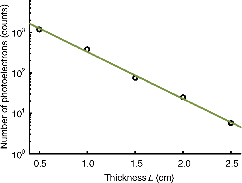$2.7 {cm}^{- 1}$ .

Figure 8 shows the simulated PDFs of the phase errors for chicken tissue samples with thicknesses ranging from 3.0 to 6.0 cm. The phase errors become more and more uniformly distributed between $- π$ and $π$ with increasing thickness. In order to quantify how these phase errors affect the performance of DOPC, we used Eq. (11) to calculate the PRB reduction coefficient $η$ as a function of sample thickness, which is shown in Fig. 9. When the sample thickness is smaller than 3.7 cm, $η$ is roughly a constant value close to 1. However, when the samples are thicker than 3.7 cm, $η$ starts to decrease exponentially. Thus, a turning point is observed around thickness $L = 3.7 cm$ , which actually corresponds to the SNR being 1. Based on Eq. (10), when the camera readout noise is much smaller than the shot noise, the expression for the SNR can be simplified to $2 \sqrt{N_{S}}$ . Since $N_{S}$ decreases exponentially with increasing sample thickness, SNR also decreases exponentially with increasing sample thickness. When the sample is thicker than 3.7 cm, the SNR becomes smaller than 1, and $η$ starts to drop exponentially and reaches 0.017 at 5.0 cm and 0.0012 at 6.0 cm. These small values of $η$ beyond the turning point demonstrate that insufficient transmitted sample light power can significantly degrade the performance of DOPC when focusing light through samples thicker than 3.7 cm.

Fig. 8

PDFs of phase errors in the simulated phase maps for chicken tissue samples with thicknesses ranging from 3.0 cm to 6.0 cm.

Fig. 9

PBR reduction coefficient $η$ and the SNR as a function of chicken tissue sample thickness.

Acknowledgments

The authors thank Dr. Puxiang Lai for helpful discussions, and Prof. James Ballard for proofreading the article. This work was sponsored in part by the National Institutes of Health Grant Nos. DP1 EB016986 and R01 CA186567.

References

1.

V. Ntziachristos, “Going deeper than microscopy: the optical imaging frontier in biology,” Nat. Methods, 7 603 –614 (2010). http://dx.doi.org/10.1038/nmeth.1483 1548-7091 Google Scholar

2.

Y. Liu, C. Zhang and L. V. Wang, “Effects of light scattering on optical-resolution photoacoustic microscopy,” J. Biomed. Opt., 17 126014 (2012). http://dx.doi.org/10.1117/1.JBO.17.12.126014 JBOPFO 1083-3668 Google Scholar

3.

L. V. Wang and H. Wu, Biomedical Optics: Principles and Imaging, Wiley-Interscience, Hoboken, New Jersey (2007). Google Scholar

4.

I. M. Vellekoop and A. P. Mosk, “Focusing coherent light through opaque strongly scattering media,” Opt. Lett., 32 2309 (2007). http://dx.doi.org/10.1364/OL.32.002309 OPLEDP 0146-9592 Google Scholar

5.

S. Popoff et al., “Measuring the transmission matrix in optics: an approach to the study and control of light propagation in disordered media,” Phys. Rev. Lett., 104 100601 (2010). http://dx.doi.org/10.1103/PhysRevLett.104.100601 PRLTAO 0031-9007 Google Scholar

6.

Z. Yaqoob et al., “Optical phase conjugation for turbidity suppression in biological samples,” Nat. Photonics, 2 110 –115 (2008). http://dx.doi.org/10.1038/nphoton.2007.297 NPAHBY 1749-4885 Google Scholar

7.

C. Stockbridge et al., “Focusing through dynamic scattering media,” Opt. Express, 20 15086 (2012). http://dx.doi.org/10.1364/OE.20.015086 OPEXFF 1094-4087 Google Scholar

8.

E. J. McDowell et al., “Turbidity suppression from the ballistic to the diffusive regime in biological tissues using optical phase conjugation,” J. Biomed. Opt., 15 025004 (2010). http://dx.doi.org/10.1117/1.3381188 JBOPFO 1083-3668 Google Scholar

9.

Y. Shen et al., “Focusing light through scattering media by full-polarization digital optical phase conjugation,” Opt. Lett., 41 1130 (2016). http://dx.doi.org/10.1364/OL.41.001130 OPLEDP 0146-9592 Google Scholar

10.

C. Ma et al., “Single-exposure optical focusing inside scattering media using binarized time-reversed adapted perturbation,” Optica, 2 869 (2015). http://dx.doi.org/10.1364/OPTICA.2.000869 Google Scholar

11.

C.-L. Hsieh et al., “Imaging through turbid layers by scanning the phase conjugated second harmonic radiation from a nanoparticle,” Opt. Express, 18 20723 (2010). http://dx.doi.org/10.1364/OE.18.020723 OPEXFF 1094-4087 Google Scholar

12.

M. Cui and C. Yang, “Implementation of a digital optical phase conjugation system and its application to study the robustness of turbidity suppression by phase conjugation,” Opt. Express, 18 3444 (2010). http://dx.doi.org/10.1364/OE.18.003444 OPEXFF 1094-4087 Google Scholar

13.

X. Xu, H. Liu and L. V. Wang, “Time-reversed ultrasonically encoded optical focusing into scattering media,” Nat. Photonics, 5 154 –157 (2011). http://dx.doi.org/10.1038/nphoton.2010.306 NPAHBY 1749-4885 Google Scholar

14.

Y. M. Wang et al., “Deep-tissue focal fluorescence imaging with digitally time-reversed ultrasound-encoded light,” Nat. Commun., 3 928 (2012). http://dx.doi.org/10.1038/ncomms1925 NCAOBW 2041-1723 Google Scholar

15.

K. Si, R. Fiolka and M. Cui, “Fluorescence imaging beyond the ballistic regime by ultrasound-pulse-guided digital phase conjugation,” Nat. Photonics, 6 657 –661 (2012). http://dx.doi.org/10.1038/nphoton.2012.205 NPAHBY 1749-4885 Google Scholar

16.

B. Judkewitz et al., “Speckle-scale focusing in the diffusive regime with time-reversal of variance-encoded light (TROVE),” Nat. Photonics, 7 300 –305 (2013). http://dx.doi.org/10.1038/nphoton.2013.31 NPAHBY 1749-4885 Google Scholar

17.

T. R. Hillman et al., “Digital optical phase conjugation for delivering two-dimensional images through turbid media,” Sci. Rep., 3 1909 (2013). http://dx.doi.org/10.1038/srep01909 SRCEC3 2045-2322 Google Scholar

18.

E. H. Zhou et al., “Focusing on moving targets through scattering samples,” Optica, 1 227 (2014). http://dx.doi.org/10.1364/OPTICA.1.000227 Google Scholar

19.

C. Ma et al., “Time-reversed adapted-perturbation (TRAP) optical focusing onto dynamic objects inside scattering media,” Nat. Photonics, 8 931 –936 (2014). http://dx.doi.org/10.1038/nphoton.2014.251 Google Scholar

20.

H. Ruan, M. Jang and C. Yang, “Optical focusing inside scattering media with time-reversed ultrasound microbubble encoded light,” Nat. Commun., 6 8968 (2015). http://dx.doi.org/10.1038/ncomms9968 NCAOBW 2041-1723 Google Scholar

21.

M. Jang et al., “Relation between speckle decorrelation and optical phase conjugation (OPC)-based turbidity suppression through dynamic scattering media: a study on in vivo mouse skin,” Biomed. Opt. Express, 6 72 (2015). http://dx.doi.org/10.1364/BOE.6.000072 BOEICL 2156-7085 Google Scholar

22.

D. Wang et al., “Focusing through dynamic tissue with millisecond digital optical phase conjugation,” Optica, 2 728 (2015). http://dx.doi.org/10.1364/OPTICA.2.000728 Google Scholar

23.

Y. Liu et al., “Optical focusing deep inside dynamic scattering media with near-infrared time-reversed ultrasonically encoded (TRUE) light,” Nat. Commun., 6 5904 (2015). http://dx.doi.org/10.1038/ncomms6904 NCAOBW 2041-1723 Google Scholar

24.

Y. Liu et al., “Bit-efficient, sub-millisecond wavefront measurement using a lock-in camera for time-reversal based optical focusing inside scattering media,” Opt. Lett., 41 1321 (2016). http://dx.doi.org/10.1364/OL.41.001321 OPLEDP 0146-9592 Google Scholar

25.

P. Lai, X. Xu and L. V. Wang, “Ultrasound-modulated optical tomography at new depth,” J. Biomed. Opt., 17 066006 (2012). http://dx.doi.org/10.1117/1.JBO.17.6.066006 JBOPFO 1083-3668 Google Scholar

26.

H. Ke et al., “Performance characterization of an integrated ultrasound, photoacoustic, and thermoacoustic imaging system,” J. Biomed. Opt., 17 056010 (2012). http://dx.doi.org/10.1117/1.JBO.17.5.056010 JBOPFO 1083-3668 Google Scholar

27.

L. V. Wang, R. E. Nordquist and W. R. Chen, “Optimal beam size for light delivery to absorption-enhanced tumors buried in biological tissues and effect of multiple-beam delivery: a Monte Carlo study,” Appl. Opt., 36 8286 (1997). http://dx.doi.org/10.1364/AO.36.008286 Google Scholar

28.

F. Le Clerc, L. Collot and M. Gross, “Numerical heterodyne holography with two-dimensional photodetector arrays,” Opt. Lett., 25 716 (2000). http://dx.doi.org/10.1364/OL.25.000716 OPLEDP 0146-9592 Google Scholar

29.

V. N. Mahajan and G.-M. Dai, “Orthonormal polynomials in wavefront analysis: analytical solution,” J. Opt. Soc. Am. A, 24 2994 (2007). http://dx.doi.org/10.1364/JOSAA.24.002994 JOAOD6 0740-3232 Google Scholar

30.

M. Azimipour, F. Atry and R. Pashaie, “Calibration of digital optical phase conjugation setups based on orthonormal rectangular polynomials,” Appl. Opt., 55 2873 (2016). http://dx.doi.org/10.1364/AO.55.002873 Google Scholar

31.

J. Brake, M. Jang and C. Yang, “Analyzing the relationship between decorrelation time and tissue thickness in acute rat brain slices using multispeckle diffusing wave spectroscopy,” J. Opt. Soc. Am. A, 33 270 (2016). http://dx.doi.org/10.1364/JOSAA.33.000270 JOAOD6 0740-3232 Google Scholar

32.

D. Pine et al., “Diffusing wave spectroscopy,” Phys. Rev. Lett., 60 1134 (1988). http://dx.doi.org/10.1103/PhysRevLett.60.1134 PRLTAO 0031-9007 Google Scholar

33.

G. Marquez et al., “Anisotropy in the absorption and scattering spectra of chicken breast tissue,” Appl. Opt., 37 798 (1998). http://dx.doi.org/10.1364/AO.37.000798 Google Scholar

34.

P. Lai, X. Xu and L. V. Wang, “Dependence of optical scattering from intralipid in gelatin-gel based tissue-mimicking phantoms on mixing temperature and time,” J. Biomed. Opt., 19 035002 (2014). http://dx.doi.org/10.1117/1.JBO.19.3.035002 JBOPFO 1083-3668 Google Scholar

35.

I. M. Vellekoop and A. P. Mosk, “Universal optimal transmission of light through disordered materials,” Phys. Rev. Lett., 101 120601 (2008). http://dx.doi.org/10.1103/PhysRevLett.101.120601 PRLTAO 0031-9007 Google Scholar

36.

M. Jang et al., “Model for estimating the penetration depth limit of the time-reversed ultrasonically encoded optical focusing technique,” Opt. Express, 22 5787 (2014). http://dx.doi.org/10.1364/OE.22.005787 Google Scholar

37.

T. J. Farrell, M. S. Patterson and B. Wilson, “A diffusion theory model of spatially resolved, steady‐state diffuse reflectance for the noninvasive determination of tissue optical properties in vivo,” Med. Phys., 19 879 (1992). http://dx.doi.org/10.1118/1.596777 Google Scholar

38.

M. Fox, Quantum Optics: An Introduction, Oxford University Press, New York (2006). Google Scholar

Biography

Yuecheng Shen received his BSc in applied physics from the University of Science and Technology of China and a PhD in electrical engineering from Washington University in St. Louis. He is currently working as a postdoctoral research associate in biomedical engineering at Washington University in St. Louis. His current research interests focus on developing new optical techniques based on stepwise wavefront shaping and optical time reversal.

Yan Liu received his BEng from Tsinghua University, China, in 2010. He is currently a PhD student of biomedical engineering at Washington University. In Prof. Lihong Wang’s group, he has worked on photoacoustic tomography, wavefront shaping, and ultrasound-modulated optical tomography. He is developing optical phase conjugation-based wavefront shaping techniques, such as time-reversed ultrasonically encoded optical focusing and time-reversed adapted perturbation optical focusing, for focusing light inside opaque scattering media such as biological tissue.

Cheng Ma received his BSc in electronic engineering from Tsinghua University, China, in 2004. He received his PhD in electrical engineering from Virginia Tech, Virginia, USA, in 2012. He then worked as a postdoctoral research associate on wavefront shaping and photoacoustic computed tomography at the Department of Biomedical Engineering, Washington University in St. Louis, Missouri, USA. Starting in May 2016, he joined the Department of Electronic Engineering of Tsinghua University, China, as an assistant professor.

Lihong V. Wang is the Gene K. Beare distinguished professor at Washington University. His book titled Biomedical Optics won the Goodman Award. He has published 437 journal articles with an h-index of 107 (>45,000 citations). His laboratory is pushing the spatiotemporal limits of optical imaging by photoacoustic tomography, wavefront engineering, and compressed ultrafast photography. He serves as the editor-in-chief of the Journal of Biomedical Optics. He was awarded OSA’s C.E.K. Mees Medal, NIH Director’s Pioneer Award, and IEEE’s Biomedical Engineering Award.

Citation Download Citation

Yuecheng Shen, Yan Liu, Cheng Ma, and Lihong V. Wang "Focusing light through biological tissue and tissue-mimicking phantoms up to 9.6 cm in thickness with digital optical phase conjugation," Journal of Biomedical Optics 21(8), 085001 (12 August 2016). https://doi.org/10.1117/1.JBO.21.8.085001

Published: 12 August 2016

Access the abstract

JOURNAL ARTICLE
8 PAGES

DOWNLOAD PAPER SAVE TO MY LIBRARY

GET CITATION

CITATIONS

Cited by 57 scholarly publications.

Explore citations on Lens.org

RIGHTS & PERMISSIONS

Get copyright permission Get copyright permission on Copyright Marketplace

KEYWORDS

Tissue optics

Wavefronts

Optical proximity correction

Scattering

Light scattering

Laser scattering

Signal to noise ratio

1.

Introduction

Fig. 1

2.

Method

Fig. 2

2.1.

Wavefront Recording

2.2.

Wavefront Reconstruction

3.

Result

3.1.

Focusing Light Through Chicken Breast Tissue

Fig. 3

3.2.

Focusing Light Through Tissue-Mimicking Phantoms

Fig. 4

4.

Discussion and Conclusion

Appendices

Appendix A:

Requirement of Laser Coherence Length in OPC Experiments

Eq. (1)

Fig. 5

Eq. (2)

Eq. (3)

Eq. (4)

Eq. (5)

Eq. (6)

Appendix B:

Effects of Phase Errors in the Measured Wavefront on the Quality of DOPC

Eq. (7)

Eq. (8)

Eq. (9)

Eq. (10)

Eq. (11)

Fig. 6

Fig. 7

Fig. 8

Fig. 9

Acknowledgments

References

Biography

Show All Keywords

Keywords/Phrases

Search In:

Publication Years