1.

Introduction

The articular cartilage benefits from a specialized extracellular matrix architecture that is optimized for weight-bearing and resisting the stress induced in articulation. The collagen fibers in cartilage are organized in a unique “arcade” like formation.¹ The fibers are oriented perpendicularly to the interface between calcified cartilage and noncalcified cartilage in the deep radial zone (or the “deep zone”), then bend in a transitional zone (or the “intermediate zone”) to be eventually parallel to the surface in the superficial zone (or the “tangential zone”). The superficial zone is thin and only takes up 10% to 20% of the total cartilage thickness. However, it plays a critical role in protecting the inner zones and maintaining proper mechanical responses for cartilage to function normally. The collagen fibers in the superficial zone are organized in a preferential orientation² to deal with the directional mechanical demand in cartilage.³ The alteration of fiber orientation in the superficial zone has been observed in early osteoarthritis.^4,5 A careful consideration of fiber orientation may also be important in clinical treatments such as osteochondral transplantation.²

Because of the importance of fiber orientation in the superficial zone of the cartilage, a technology that can directly visualize the collagen organization would be valuable to both basic research and clinical practice. The “split-line” method has been used to reveal fiber orientation on the cartilage surface.^6,7 Split-lines are the cracks created on the articular cartilage surface when pricking the cartilage using a fine needle. These cracks are caused by the collagen fibers splitting along the lines of tensile stress, which are aligned with the collagen fibers in the superficial layer as revealed in scanning electron microscopy (SEM) studies.⁸ The collagen fibrils resisted strains better along the split-line directions than perpendicular to the split-lines.⁹

Although the “split-line” method can reveal the global fiber orientation in the superficial zone of the cartilage, it is destructive and impractical for diagnosis purpose. Clinical imaging technologies such as magnetic resonance imaging (MRI) are nondestructive, but their current resolution is insufficient to resolve the detailed structural features in the thin cartilage.¹⁰ High-resolution microscopic MRI (μMRI)¹¹ is promising for differentiating histological zones in cartilage. However, current $\mu \mathrm{MRI}$ hardware is only limited to imaging prepared small samples. Small angle x-ray scattering (SAXS)¹² was also explored to obtain collagen orientation in cartilage from the side of the sample; but special x-ray facility such as synchrotron radiation¹² is often needed in SAXS. Currently, polarization light microscopy (PLM) is recognized as the primary tool to detect fiber orientation in cartilage.^13,14 The highly organized collagen structure in cartilage produces a strong optical birefringence, which can be detected using polarized light. Unfortunately, PLM has limited imaging depth and can only image prepared thin cartilage sections from the cross sectional side. PLM cannot image collagen fiber orientation in intact cartilage from the synovial surface.

Optical coherence tomography (OCT) is an emerging high-resolution nondestructive three-dimensional (3-D) optical imaging technology.¹⁵ OCT achieved micrometer scale resolution and can detect structural and morphological changes in cartilage as well as surface roughness associated with osteoarthritis.^16–19 Because of the presence of optical birefringence in cartilage, polarization-sensitive OCT (PSOCT) has also been widely applied in cartilage imaging.^20,21 A common finding in many PSOCT studies was the “banding” pattern in images of normal cartilage due to birefringence, which disappeared in cartilage with progressive degeneration.²² Therefore, the loss of birefringence can be used as a biomarker for detecting early cartilage degeneration.²³

Despite its great potential for nondestructive cartilage imaging, very few PSOCT studies investigated the possibility of imaging the fiber orientation in cartilage. It is known that the optic axis measured in PSOCT is related to the fiber orientation. Unfortunately, conventional PSOCT only measures the “cumulative” optic axis that represents the integrated signal from the tissue surface to a particular imaging depth. Such integrated optic axes do not represent the actual fiber orientation.²⁴ It has recently been shown that the 3-D fiber orientation in cartilage can be obtained by analyzing the depth profiles of tissue birefringence²⁵ or optic axis²⁶ when evaluated at multiple different incident angles. However, only single point measurement was achieved in these early studies^26,27 and thus it is challenging to apply these approaches to obtain the spatial- and depth-resolved orientation in the whole cartilage.

Optical polarization tractography (OPT) was a newly developed method for imaging fiber orientation in tissue. It utilized a Jones calculus based method to extract the true “local” optic axis from PSOCT measurements.^28,29 Validation studies have shown that OPT achieved histology-like accuracy in imaging fiber orientation in tissues.³⁰ As an optical polarization based method, OPT can image the fiber orientation and birefringence at the sample surface as in conventional PLM. However, OPT can nondestructively image fiber orientation and birefringence at different depths from the tissue surface, which is not feasible in PLM. Recent studies have demonstrated that OPT can be potentially applied to image fiber structures in skeletal muscle,³¹ heart muscle,³² and blood vessels.³³ In this study, we showed that OPT can image collagen fiber orientation in the superficial layer of the articular cartilage. The fiber orientation measured in OPT agreed very well with those obtained using the standard split-line procedure. In addition, the superficial zone thickness can also be estimated using the depth profile of the local birefringence obtained in OPT.

2.

Method

3.

Results

Figure 1 shows example image data obtained from OPT scanning. Figure 1(a) shows a photograph of split-line patterns created on a cartilage sample. Due to the ink staining, the split-lines are clearly visible on the cartilage surface. The orientation of all split-lines formed a general converging pattern from the side toward the groove. The marked square in Fig. 1(a) (a $6{\mathrm{mm}}^2\times 6{\mathrm{mm}}^2$ area) indicates the OPT scanning area. Figure 1(b) shows the 3-D intensity image of the sample obtained in OPT. The A-, B-, and C-scan directions were marked using arrows in Figs. 1(a) and 1(b). The split-lines are also visible in the intensity image.

Fig. 1

Example OPT images of an articular cartilage sample. (a) A photograph of the split-line pattern at the cartilage surface. The dash-line box indicates the $6{\mathrm{mm}}^2\times 6{\mathrm{mm}}^2$ OPT image area. (b) The 3-D intensity image of the sample volume. A sagittal (C-scan) cutting plane is illustrated with marked directions of A-, B-, and C-scan. Also shown are the corresponding cross sectional images of (c) intensity, (d) color-coded local optic axis, and (e) local birefringence at the sagittal cutting plane marked in (b). (f) A histology image (H&E stain) of the same cartilage sample. A zoom-in view of a small section [box in (f)] was shown in (g). SZ, superficial zone; TZ, transitional zone; and RZ, radial zone.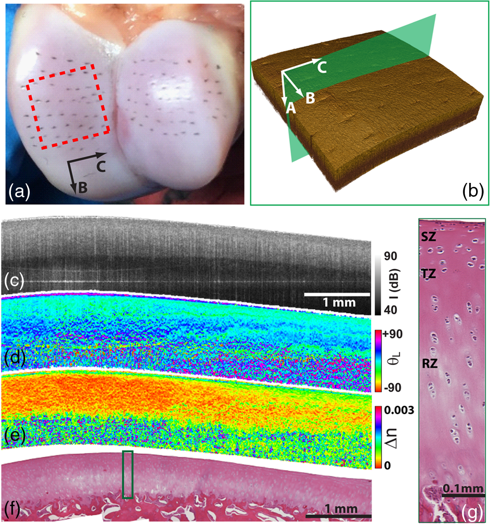

Figures 1(c), 1(d), and 1(e) show representative cross sectional images of the intensity, color-coded local optic axis, and local birefringence. These cross sectional images were constructed from a sagittal cutting plane as shown in Fig. 1(b). The cartilage body had a stronger intensity than the underneath calcified cartilage/bone. The cartilage was thicker at the left end than the right end (toward the groove). The cartilage thickness can be identified from the intensity image as shown previously.¹⁶ The fiber orientation was relatively homogeneous close to the surface, but showed a large variation in the calcified cartilage/bone region [Fig. 1(d)]. The birefringence appeared in green color within a very thin layer right underneath the surface. Then the birefringence decreased in value in the radial zone (yellow color), and increased significantly (blue color) in the bone region [Fig. 1(e)]. Similar to the fiber orientation, the birefringence was significantly noisier in the calcified/bone region. The noisy and high birefringence values in the bone region may be caused by the low signal intensity [Fig. 1(c)].

The general cartilage morphology shown in the histology [Fig. 1(f)] agreed well with that obtained in the intensity image [Fig. 1(c)]. From a magnified small histology section [marked on Fig. 1(f)], different cartilage zones can be roughly visualized based on the morphology of the chondrocytes. In the superficial zone (SZ), chondrocytes appeared as flattened ellipsoids that were tangential to the cartilage surface. The spheroidal shaped chondrocytes appeared to be arranged perpendicular toward the cartilage surface in the radial zone (RZ). However, a precise boundary between different zones was elusive from the H&E histology.

The fiber orientations can be better visualized in the en face plane at different depths from the cartilage surface [Fig. 2]. As a reference, the corresponding images of OPT intensity and birefringence were also presented. These images were extracted from the 3-D OPT volumes ($6.0{\mathrm{mm}}^3\times 6.0{\mathrm{mm}}^3\times 1.14{\mathrm{mm}}^3$) obtained in the same sample shown in Fig. 1. The split-lines were clearly visible in the en face intensity images. The orientation of the split-lines stayed the same over the entire depth. However, the fiber orientation obtained in the OPT varied over depth. At $52\text{-}\mu \mathrm{m}$ depth, the streamlines in the top half of the image had negative angles; whereas the bottom half showed positive angles. At $152\text{-}\mu \mathrm{m}$ depth, most of the streamlines appeared to be horizontal. Then at $400\text{-}\mu \mathrm{m}$ depth, most of fibers were aligned in the positive direction. The OPT orientation measured at $52\text{-}\mu \mathrm{m}$ depth appeared to be most similar to the split-line results.

Fig. 2

The $6{\mathrm{mm}}^2\times 6{\mathrm{mm}}^2$ en face tractographic images extracted at different depths from the OPT image volume as shown in Fig. 1(a). The corresponding intensity images showing the split-lines and the birefringence images are shown in the second and third columns, respectively. These images were extracted from the 3-D OPT volumes ($6.0{\mathrm{mm}}^3\times 6.0{\mathrm{mm}}^3\times 1.14{\mathrm{mm}}^3$) obtained in the same sample shown in Fig. 1.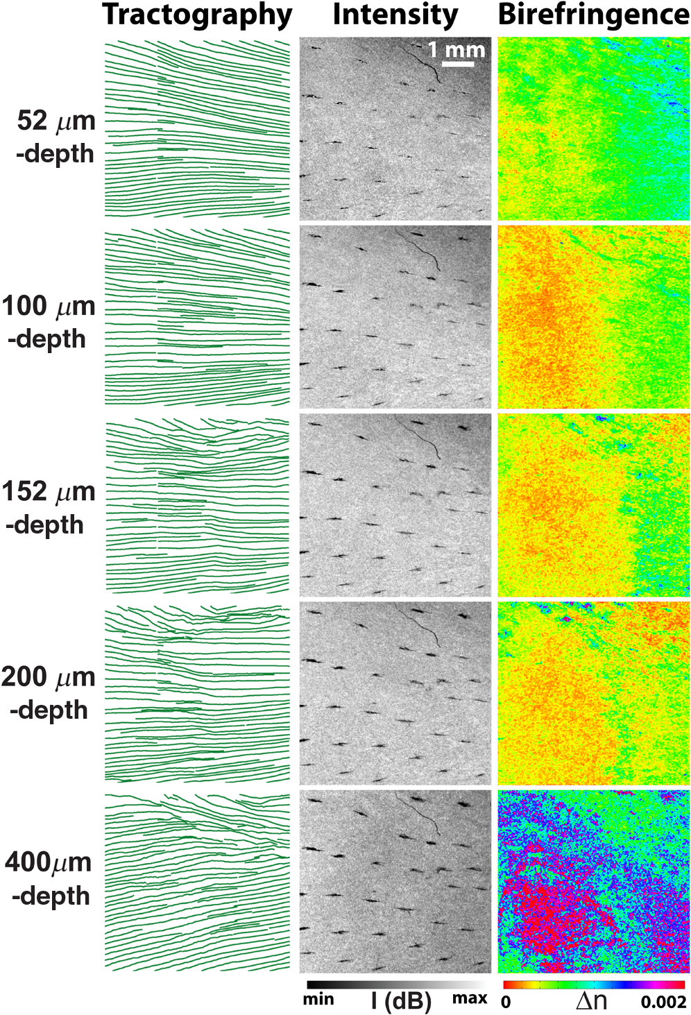

Figure 2 shows that the tissue birefringence varied over the depth in cartilage when examined in the en face planes. This observation is consistent with that from the cross sectional images [Fig. 1]. The color-coded birefringence image appeared in blue-purple color at $400\text{-}\mu \mathrm{m}$ depth that was inside the calcified cartilage/bone region. Within the region of noncalcified cartilage, the birefringence appeared to decrease initially because it had a smaller value at $100\text{-}\mu \mathrm{m}$ depth than at $52\text{-}\mu \mathrm{m}$ depth. It then remained about the same from 100 to $200\text{-}\mu \mathrm{m}$. As elaborated in the discussions, such depth-dependent birefringence profiles within the cartilage are likely attributed to “arcade” fiber structure in the noncalcified cartilage as the fibers become more aligned (or “isotropic”) with the incident light in the radial zone.

Figure 3 showed a quantitative comparison between the fiber orientation measured in OPT and the split-lines angles in this cartilage sample (Fig. 1). The orientation of each split-line was quantified and represented using a short line segment [Fig. 3(b)]. The fiber orientations obtained in OPT at $56\text{-}\mu \mathrm{m}$ depth were shown as solid lines in the same figure along with the fitted split-line segments. As shown in Fig. 3(c), the two methods agreed very well with each other and were highly correlated ($R^2=0.94$).

Fig. 3

(a) The image of split-lines obtained from averaged intensity images from 0 to $200\mu \mathrm{m}$ in depth. (b) The fitted split-lines (short line segments) and OPT results extracted at $56\text{-}\mu \mathrm{m}$ depth (solid lines in green). (c) The correlation between fiber orientations measured from split-lines and OPT using data shown in (b). (d) The coefficient of determination ($R^2$) obtained from the correlation between split-lines and OPT at different depths. Also shown is the depth profile of the overall error [Eq. (2)] between the angles measured in split-lines and OPT.

Because the fiber orientation measured in OPT changed with depth (Fig. 2), the correlation between OPT and split-lines was also depth dependent [Fig. 3(d)]. The coefficient of determination of the correlation ($R^2$) increased from 0.4 at surface to 0.94 at depth $56\mu \mathrm{m}$ and then decreased to $\sim 0.5$ at $200\text{-}\mu \mathrm{m}$ depth. The $R^2$ remained more than 0.8 between $44\mu \mathrm{m}$ and $96\mu \mathrm{m}$ in depth. Accordingly, the overall RMSE between the OPT orientation and split-line angles reached a minimum of 0.58 deg at $56\mu \mathrm{m}$ depth. The error was consistently low ($<1\mathrm{deg}$) between 44 and $100\mu \mathrm{m}$ in depth.

Similar results were obtained from split-lines obtained in other cartilage samples. Figure 4 shows the correlation between OPT and split-lines obtained in all five samples with a total of 112 split-lines. Figure 4(a) shows the correlation between split-line and OPT measurements at the depth of $56\mu \mathrm{m}$. The correlation result had a high $R^2$ of 0.95, a very close to 1.0 slope, and a small intercept of $\sim 0.4\mathrm{deg}$, all indicating an excellent agreement between the two measurements. Further analysis indicated that the difference between the angles obtained in split-line and OPT was less than or equal to 5 deg in more than 89% of the split-lines [Fig. 4(b)]. Figure 4(c) shows the coefficient of determination ($R^2$) and overall error calculated from the correlation between split-lines and OPT at different depths. The $R^2$ stayed above 0.9 using OPT results measured at depths between 40 and $108\mu \mathrm{m}$; whereas the corresponding overall RMSE was $<0.5\mathrm{deg}$ between the two methods.

Fig. 4

(a) The correlation between the split-line orientation and OPT in all cartilage samples (a total of 112 split-lines). The OPT results were extracted at the depth of $56\mu \mathrm{m}$. (b) The distribution of the difference in orientation measured from split-lines and OPT. The line curve shown is a Gaussian fitting of $y=12.17\exp [-{(x-0.47)}^2/22.4]$ with $R^2=0.86$ and $\mathrm{RMSE}=1.68$. 89.3% of the split-lines had a $\le 5\mathrm{deg}$ angle difference from the OPT results. (c) The coefficient of determination ($R^2$) of the correlation between all split-lines and OPT as well as the overall error [Eq. (2)] calculated at different depths.

4.

Discussion

Despite being a destructive method, the split-line procedure was the only currently available way to map the global fiber orientation on the whole cartilage surface. Our results indicated that the fiber orientation measured in OPT was highly consistent with the split-line results. In addition to being a nondestructive imaging method, OPT also provides a continuous map of the fiber orientation on the entire cartilage surface; whereas the split-lines can be produced only at discrete locations.

However, it is important to understand why only the OPT results obtained at depths between $\sim 40$ and $108\mu \mathrm{m}$ showed excellent agreement with the split-line results. The lower limit of $\sim 40\mu \mathrm{m}$ is likely due to special structures in the superficial layer of the cartilage. Studies have shown that additional microscopic structures exist at the “most superficial” layer of the superficial zone.^1,35 This special layer may extend $\sim 15\text{-}\mu \mathrm{m}$ deep into the superficial layer and have different tissue composition and morphology. Fiber orientation changes inside the superficial zone were also observed in both PLM³⁶ and SEM studies.³⁷ It is possible that the split-line orientation was less influenced by this “most superficial” layer of the superficial zone.

The upper depth limit of $\sim 100\mu \mathrm{m}$ obtained in the correlation analyses was likely determined by the thickness of the superficial zone.^1,14 The OPT only measures the fiber orientation in an “evaluation plane” that is perpendicular to the incident light.³⁰ When the fibers start to arch in the transitional zone toward the perpendicular orientation in the deep zone, their projections in the evaluation plane also changed. We noticed that the sample birefringence (Figs. 1 and 2) appeared to reach a minimum at $\sim 100\mu \mathrm{m}$, suggesting the fibers may have become perpendicular to the surface at this depth.

To investigate this further, the cartilage sample was cut to reveal the internal cross section of the sample and OPT was applied to image it directly from the side. Such a “side-scan” scheme was similar to the conventional PLM imaging of the cross sectional cartilage samples^11,14 where the superficial zone can be readily resolved (Fig. 5). In particular, the streamlines [Fig. 5(c)] clearly revealed the “arcade” like architecture in different zones. As a color-coded representation of the same cross sectional axis image, Fig. 5(b) showed a blue layer at small depths that indicated a close to zero-degree orientation in the superficial zone. As a comparison, Fig. 5(d) shows the “top-scan” birefringence images obtained at the same location. The “top-scan” results were obtained by imaging the cartilage from the synovial surface as in the previous figures.

Fig. 5

The OPT results of intensity (a), optic axis (b), and tractography (c) obtained from the side of the cartilage sample (the “side-scan”). (d) The birefringence image of the same sample obtained from the cartilage surface (the “top-scan”). (e) The quantitative depth profiles of the fiber orientation (from the “side-scan”) and birefringence (from the “top-scan”) obtained from a ROI as marked in (b) and (d). The solid line on the fiber orientation curve is the fitting results using the hyperbolic tangent function. The dashed line labeled as “SZ” marks the boundary of the superficial zone.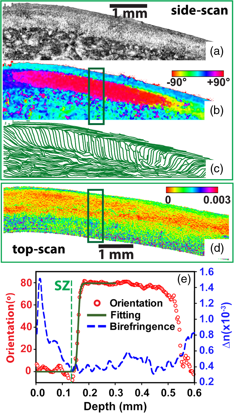

Figure 5(e) shows a comparison between the quantified one-dimensional (1-D) depth profiles of the side-scan fiber orientation and top-scan birefringence. These curves were calculated by averaging all 1-D scans from a ROI ($400\text{-}\mu \mathrm{m}$ wide) marked in Figs. 5(b) and 5(d). The depth in Fig. 5(e) was calculated assuming an optical refractive index of 1.5 as reported in a previous study.¹⁶ The side-scan orientation curve can be well fitted using the hyperbolic tangent function as described by Xia et al.¹¹ The superficial zone boundary was determined at the depth where the orientation changed more than 1 deg, which resulted in a superficial layer thickness of $\sim 142\mu \mathrm{m}$ at this location.

The aforementioned superficial zone thickness determined from the “side-scan” coincided with the depth where the “top-scan” birefringence was about to reach the baseline [Fig. 5(e)]. In addition, the birefringence reached the maximum at $\sim 14\text{-}\mu \mathrm{m}$ depth, which coincided with the thickness of the “most superficial” layer reported in a previous study.³⁵ The middle 1/3 of the depth between the maximum and the first minimum of the birefringence was about 50 to $90\mu \mathrm{m}$, from which the OPT results showed consistent agreement with the split-line results. This observation can serve as an empirical rule to determine the best depth when applying OPT to image fiber orientation in the superficial zone of the cartilage.

The birefringence measured in OPT represents the true birefringence only when the collagen fibers are perpendicular to the incident light,²⁵ which is valid in the superficial zone. However, the collagen fibers are almost perpendicular to the cartilage surface in the radial zone, where the fibers appear more “isotropic” to the incident light. Therefore, the measured birefringence appeared to be very small within the radial zone. Similarly, OPT measures the true fiber orientation in the superficial zone where the fibers are tangential to the cartilage surface. The fiber orientations measured in the radial zone only represent the projected fiber orientation within the plane perpendicular to the incident light.³⁰

The birefringence depth profile obtained from the top-scan OPT provides a nondestructive way to estimate the thickness of the superficial zone. As shown in Fig. 5(e), the superficial zone coincided with the depth where the top-scan birefringence started to approach its baseline. Applying this criterion to other locations of the same cartilage, we obtained an average superficial zone thickness of $130\mu \mathrm{m}\pm 16\mu \mathrm{m}$ for this cartilage sample. As shown previously,¹⁶ the thickness of the whole noncalcified cartilage can be obtained from the intensity image. Therefore, the OPT can potentially measure both the cartilage thickness and its superficial zone thickness in addition to the fiber orientation in the superficial zone.

5.

Conclusion

We showed in this study that OPT provides a nondestructive way for visualizing fiber orientation in the superficial zone of fresh cartilage. In addition, the depth-resolved image of the tissue birefringence obtained in OPT can be used to assess the thickness of the superficial zone. Although only porcine phalangeal cartilage was tested in this study, we hypothesize that our results and analyses are still applicable when applying OPT to other cartilage samples. The basic fiber architecture in cartilage has been reported to be similar in several different species.¹ Nevertheless, additional studies are necessary to fully understand the capability and limitation of using the OPT technology in cartilage imaging.