1.

Introduction

Quantitative photoacoustic tomography (PAT) is concerned with recovering quantitatively accurate estimates of chromophore concentration distributions, or related quantities such as optical coefficients or blood oxygenation, from photoacoustic images.¹ The source of contrast in PAT is optical absorption, which is directly related to the tissue constituents. By obtaining PAT images at multiple optical wavelengths, it may be possible to recover chemically specific information about the tissue. However, such a spectroscopic use of PAT images must consider the effect of the spatially and spectrally varying light fluence distribution. As a photoacoustic image is the product of the optical absorption coefficient distribution, which carries information about the tissue constituents, and the optical fluence, which only acts to distort that information, the challenge in quantitative photoacoustic imaging is to remove the effect of the light fluence.

A common approach is to use a model of the unknown fluence and use it to extract the desired optical properties from the measured data. This has been done analytically^2–5 or numerically,^6,7 often within a minimization framework.^8–15 The majority of this literature uses the diffusion approximation to the radiative transfer equation (RTE) to model the light distribution, which is accurate in highly scattering media.¹⁶ In PAT, the region of interest often lies close to the tissue surface where the diffusion approximation is not accurate. The RTE, on the other hand, is widely considered to be an accurate model of light transport so long as coherent effects are negligible, which is the case here. Finite element discretizations of the RTE have been developed^17–21 and proposed for quantitative PAT reconstructions,^12,15 but due to the need to discretize in angle as well as space, they quickly become computationally intensive and their applicability is limited to small- and medium-scale problems. An alternative is Monte Carlo (MC) modeling,^22,23–25 which is a stochastic technique for modeling light transport that converges to the solution to the RTE. The significant advantage of the MC approach is that it is highly parallelizable, thus it scales well to the large-scale inversions that will be encountered in practice.

MC models of light transport are popular in biomedical optics and have predominantly been applied in the planning of the experimental measurements^26–28 and in dosimetric studies for a range of light-based therapies.^29–31 Many of the applications are summarized by Zhu et al.³² One early MC model of light transport, MCML,²² computes the fluence in three-dimensional (3-D) slab geometry. This model was later extended to simulate spherical inclusions in the tissue,³³ and later to spheroidal and cylindrical³⁴ inclusions. MC modeling in 3-D heterogeneous media has been shown both for voxelized media,²³ which was later GPU-accelerated,²⁴ and using a mesh-based geometry.^25,35 Although the RTE is an equation for the radiance, which is a function of angle at every point, the quantity usually calculated by MC models is the fluence rate, which is the radiance integrated over all angles. The reasons are practical: most measurable quantities are related to the fluence rate rather than the radiance, storing just the integrated quantity saves on computational memory, and the estimates for the fluence rate will converge sooner than the underlying estimates for the radiance. In photoacoustics, the measurable signal is related to the fluence (the time-integrated fluence rate) so current MC models can be used in the simulation of photoacoustic signals. However, as will be discussed in Sec. 4, the full angle-dependent radiance is required when tackling the inverse problem of estimating the optical coefficients, specifically the optical scattering. A common approach in estimating the optical coefficients is to use a gradient-based inversion scheme in which functional gradients are used to minimize some objective function. This paper demonstrates the computation of these gradients through the use of forward and adjoint MC models of the radiance.

In this paper, Sec. 2 introduces the inverse problem of quantitative PAT. Sections 3 and 4 present forward and adjoint MC models of the radiance employing a harmonic angular basis. In Sec. 5, it is shown that this choice of basis allows the functional gradients for the inverse problem to be calculated straightforwardly. Inversions for absorption and scattering coefficient distributions are given in Sec. 6.

2.

Quantitative Photoacoustic Tomography

The inverse problem in QPAT can be stated as the minimization

3.

Monte Carlo Modeling of Light Transport

In PAT, the optical and acoustic propagation times are so different that the optical propagation can be considered instantaneous and the time-dependence of the light transport can be neglected. The time-independent RTE is given by

By calculating photon paths through the medium, the MC models presented in the literature^22–24,35 do in fact simulate the radiance, but this is typically integrated over angle upon deposition of the weights in the voxels. In order to simulate the radiance, a method of depositing the weight in the voxels without losing the angular information is required.

3.2.

Validation of the Forward Model

Analytical solutions to the RTE are available for the fluence for a range of geometries and source types;^23,42,43 however, there are few analytical solutions for the radiance, particularly in 2-D. The RMC model was compared to one such analytic solution for an infinite, homogeneous 2-D domain illuminated by an isotropic point source.^44–46 An isotropic point source was placed at the center of a domain of size $15\mathrm{mm}\times 15\mathrm{mm}$, large compared to the transport mean free path in order to approximate an infinite domain. The absorption and scattering coefficients were 0.01 and $10{\mathrm{mm}}^{-1}$, respectively, and the Henyey–Greenstein phase function⁴⁷ was used with $g$ set to 0.9. The pixel size was $0.05\mathrm{mm}\times 0.05\mathrm{mm}$, and five Fourier harmonics were used. Figure 1 shows the good agreement between the analytical and RMC modeled radiance at radial distances of 2 and 3 mm from the source along the horizontal axis.

Fig 1

Polar plots of the angle-resolved radiance due to an isotropic point source in a homogeneous domain with ${\mu }_{\mathrm{a}}=0.01{\mathrm{mm}}^{-1}$, ${\mu }_{\mathrm{s}}=10{\mathrm{mm}}^{-1}$, and $g=0.9$. Results from an analytic method (infinite domain) and RMC simulations ($15\mathrm{mm}\times 15\mathrm{mm}$ square domain) shown.

4.

Adjoint Monte Carlo Model

The adjoint equation to the RTE is given by

4.1.

Validation of the Adjoint Model

The adjoint model was validated by checking that it satisfied the condition

Eq. (13)

$$⟨\mathcal{G}\mathbf{u},\mathbf{v}⟩=⟨\mathbf{u},{\mathcal{G}}^{*}\mathbf{v}⟩,$$

where $\mathcal{G}$ and ${\mathcal{G}}^{*}$ are the (Green’s) operators solving the corresponding forward and adjoint RMC models, and $\mathbf{u}$ and $\mathbf{v}$ are the angle and position dependent source and detector, i.e.,

Eq. (14)

$$\phi (\mathbf{r},\widehat{\mathbf{s}})=\mathcal{G}\mathbf{u}\iff \mathcal{L}\phi =\mathbf{u},{\phi }^{*}(\mathbf{r},\widehat{\mathbf{s}})={\mathcal{G}}^{*}\mathbf{v}\iff {\mathcal{L}}^{*}{\phi }^{*}=\mathbf{v}.$$

Let $\mathbf{u}={\rho }_{\mathrm{s}}(\mathbf{r}){\mathrm{\Theta }}_{\mathrm{s}}(\widehat{\mathbf{s}})$, $\mathbf{v}={\rho }_{\mathrm{d}}(\mathbf{r}){\mathrm{\Theta }}_{\mathrm{d}}(\widehat{\mathbf{s}})$ and consider three different cases

$$\begin{gathered} \text{Case}1:(\text{isotropic source and detector}){\mathbf{u}}_1=\delta (\mathbf{r}-{\mathbf{r}}_s)/2\pi ,{\mathbf{v}}_1=\delta (\mathbf{r}-{\mathbf{r}}_d)/2\pi . \\ \text{Case}2:(\text{isotropic source},\text{angular detector}){\mathbf{u}}_2=\delta (\mathbf{r}-{\mathbf{r}}_s)/2\pi ,{\mathbf{v}}_2=\delta (\mathbf{r}-{\mathbf{r}}_d){\mathrm{\Theta }}_{\mathrm{d}}(\widehat{\mathbf{s}}). \\ \text{Case}3:(\text{spatial source},\text{angular detector}){\mathbf{u}}_3={\rho }_{\mathrm{s}}(\mathbf{r}){\mathrm{\Theta }}_{\mathrm{s}}(\widehat{\mathbf{s}}),{\mathbf{v}}_3=\delta (\mathbf{r}-{\mathbf{r}}_d){\mathrm{\Theta }}_{\mathrm{d}}(\widehat{\mathbf{s}}). \end{gathered}$$

Substituting these into Eq. (13) yields

Eq. (15)

$${\mathrm{\Phi }}_1({\mathbf{r}}_d)={\mathrm{\Phi }}_1^{*}({\mathbf{r}}_s),$$

Eq. (16)

$${\int }_{2\pi }{\phi }_2({\mathbf{r}}_d,\widehat{\mathbf{s}}){\mathrm{\Theta }}_{\mathrm{d}}(\widehat{\mathbf{s}})\mathrm{d}\widehat{\mathbf{s}}={\mathrm{\Phi }}_2^{*}({\mathbf{r}}_s),$$

Eq. (17)

$${\int }_{2\pi }{\phi }_3({\mathbf{r}}_d,\widehat{\mathbf{s}}){\mathrm{\Theta }}_{\mathrm{d}}(\widehat{\mathbf{s}})\mathrm{d}\mathbf{r}={\int }_{2\pi }{\int }_{\mathrm{\Omega }}{\phi }_3^{*}(\mathbf{r},\widehat{\mathbf{s}}){\rho }_{\mathrm{s}}(\mathbf{r}){\mathrm{\Theta }}_{\mathrm{s}}(\widehat{\mathbf{s}})\mathrm{d}\widehat{\mathbf{s}},$$

where ${\phi }_{1,2,3}$ and ${\phi }_{1,2,3}^{*}$ are the forward and adjoint radiances from computing $\mathcal{G}{\mathbf{u}}_{1,2,3}$ and ${\mathcal{G}}^{*}{\mathbf{v}}_{1,2,3}$, respectively. $\mathrm{\Phi }$ is the fluence or angle-integrated radiance. It can be seen from Eq. (15) that case 1, where a pair of isotropic $\delta$-functions are used for ${\mathbf{u}}_1$ and ${\mathbf{v}}_1$, that we expect the resulting fluence values at their respective positions, ${\mathrm{\Phi }}_1({\mathbf{r}}_d)$ and ${\mathrm{\Phi }}_1^{*}({\mathbf{r}}_s)$, to be equal. This is an intuitive result given the reciprocity of the RTE and the angular independence of the source-detector combination.

Simulations were performed using a $40\mathrm{mm}\times 40\mathrm{mm}$ ($101\times 101\text{pixel}$) domain, and 10 Fourier harmonics. Each source distribution emitted ${10}^6$ photons. ${\mathbf{r}}_s$ was set to be the center of the domain with ${\mathbf{r}}_d$ moved along the $x$-direction across the domain. Comparisons are shown in Fig. 2 for case 1 with an isotropic source and detector, Fig. 3 for case 2 with an isotropic source and anisotropic detector with ${\rho }_{\mathrm{d}}=\delta (\mathbf{r}-{\mathbf{r}}_s)$, ${\mathrm{\Theta }}_{\mathrm{d}}=\frac{1}{\pi }{\sin }^2(2\theta )$, and Fig. 4 for case 3 with the same ${\rho }_{\mathrm{d}}$, ${\mathrm{\Theta }}_{\mathrm{d}}$ but with istropic ${\mathrm{\Theta }}_{\mathrm{s}}$ and the distributed ${\mathrm{\Theta }}_{\mathrm{s}}(\mathbf{r})$ shown in Fig. 4(a). Good agreement was obtained in all cases, showing the the RMC adjoint model is an accurate representation of the RTE adjoint. It can be seen in the comparison of $⟨\mathcal{G}{\mathbf{u}}_{1,2,3},{\mathbf{v}}_{1,2,3}⟩$ with $⟨{\mathbf{u}}_{1,2,3},{\mathcal{G}}^{*}{\mathbf{v}}_{1,2,3}⟩$ that some noise is present in the latter. As the overall number of photons simulated in the forward and adjoint simulations was the same, the use of spatially distributed sources in the adjoint case resulted in lower photon density in the domain, thereby reducing SNR. This issue was exacerbated in the case where an angularly dependent detector was used because a significant fraction of photons went undetected.

Fig. 2

Plot of $⟨\mathcal{L}{\mathbf{u}}_1,{\mathbf{v}}_1⟩$ and $⟨{\mathbf{u}}_1,{\mathcal{L}}^{*}{\mathbf{v}}_1⟩$ to validate the adjoint model. ${\mathbf{u}}_1$ and ${\mathbf{v}}_1$ were isotropic point sources with ${\mathbf{u}}_1$ at the center of the domain and ${\mathbf{v}}_1$ translated across the domain at $y=23.6\mathrm{mm}$.

Fig. 3

(a) Polar plot of source distribution for ${\mathbf{v}}_2=\delta (\mathbf{r}-{\mathbf{r}}_s)\frac{1}{\pi }{\sin }^2(2\theta )$; (b) plot of $⟨\mathcal{L}{\mathbf{u}}_2,{\mathbf{v}}_2⟩=⟨{\mathbf{u}}_2,{\mathcal{L}}^{*}{\mathbf{v}}_2⟩$ for validation of adjoint model. Plot was produced with ${\mathbf{u}}_2$ as an isotropic point source at the center of the domain. ${\mathbf{v}}_2$ was translated across the domain along a line at $y=23.6\mathrm{mm}$.

Fig. 4

(a) Isotropic source distribution ${\mathbf{u}}_3=P_s(\mathbf{r})$; (b) $⟨\mathcal{L}{\mathbf{u}}_3,{\mathbf{v}}_3⟩$ and $⟨{\mathbf{u}}_3,{\mathcal{L}}^{*}{\mathbf{v}}_3⟩$ to validate the adjoint model. ${\mathbf{v}}_3$ was an anisotropic point source emitting light over angle following $\frac{1}{\pi }{\sin }^2(2\theta )$. ${\mathbf{v}}_3$ was translated along a line across the domain at $y=23.6\mathrm{mm}$, as shown by the gray line dashed line in (a).

5.

Functional Gradients

Both the radiance and the adjoint radiance can be expressed as Fourier series as in Eq. (8). By substituting these expressions into Eqs. (3) and (4) for the functional gradients, simple and easily computed expressions for the gradients can be obtained. The fluence is simply given by the isotropic component of the field $a_0$. The other terms in the expressions for the functional gradients contain integrals of products of the radiance and its adjoint. If $a_0^{*}$, $a_n^{*}$, and $b_n^{*}$ are the Fourier coefficients of the adjoint radiance, then the gradient with respect to absorption can be written as

The second term in Eq. (4) is

6.

Inversions for Absorption and Scattering

The forward and inverse MC models of radiance described above were used with a gradient-descent (GD) scheme to estimate ${\mu }_{\mathrm{a}}(\mathbf{x})$ and ${\mu }_{\mathrm{s}}(\mathbf{x})$ from simulated PAT images by minimizing the error functional in Eq. (2). As the adjoint source, $q^{*}(\mathbf{x},\widehat{\mathbf{s}})={\mu }_{\mathrm{a}}(\mathbf{x})[H^{\text{meas}}(\mathbf{x})-H(\mathbf{x})]$ was independent of angle, photons were launched istropically with the launch position being spread out over the range of a source voxel using a randomly distributed number on the interval [0, 1]. The initial photon weight was scaled according to the source strength with normalization of the output quantity (i.e., radiance, absorbed energy density, and harmonic) being $N_p$. The adjoint source may be negative in some places, so the initial photon weight is negative and weight deposition is also negative. The photon termination condition was, therefore, set to be the absolute value of the photon weight falling below the threshold value. The gradients were calculated using Eqs. (20) and (26). A GD scheme was chosen for the minimization because it is more robust to the MC noise in the functional gradients and error functional than techniques such as L-BFGS that use second-order information. A line-search algorithm presented by Hager and Zhang⁴⁸ was used for the reconstruction of ${\mu }_{\mathrm{a}}$. A backtracking line search was implemented for the reconstruction of ${\mu }_{\mathrm{s}}$. This is described in Sec. 6.2.

The termination condition used by the optimization was

6.1.

Inversion for Absorption Coefficient

The domain used in the estimation of the absorption coefficient consisted of a background absorption coefficient of $0.01{\mathrm{mm}}^{-1}$ with a rectangular inclusion equal to $0.2{\mathrm{mm}}^{-1}$ [shown in Fig. 5(a)], and a background scattering coefficient of $5{\mathrm{mm}}^{-1}$ with a rectangular inclusion equal to $15{\mathrm{mm}}^{-1}$ [shown in Fig. 5(b)]. The anisotropy was a homogeneously distributed value of 0.9. The measured data, $H^{\text{meas}}$, were formed using an MC simulation illuminated by a collimated line source on the boundary at $z=0\mathrm{mm}$ and on the adjacent boundary at $x=4\mathrm{mm}$, consisting of ${10}^8$ photons. The inversion for the absorption coefficient only was performed under the assumption that the scattering coefficient was known and the starting estimate of the absorption coefficient was a homogeneous value of $0.01{\mathrm{mm}}^{-1}$. The termination condition in Eq. (27) was satisfied after 11 iterations, having taken 4.1 h to run, and is shown in Fig. 5(b) with profiles through the true and reconstructed distributions of ${\mu }_{\mathrm{a}}$ shown in Fig. 5(d).

Fig. 5

(a) True absorption coefficient, (b) true scattering coefficient, (c) reconstructed absorption coefficient after nine iterations, (d) profiles through true and reconstructed absorption coefficient at 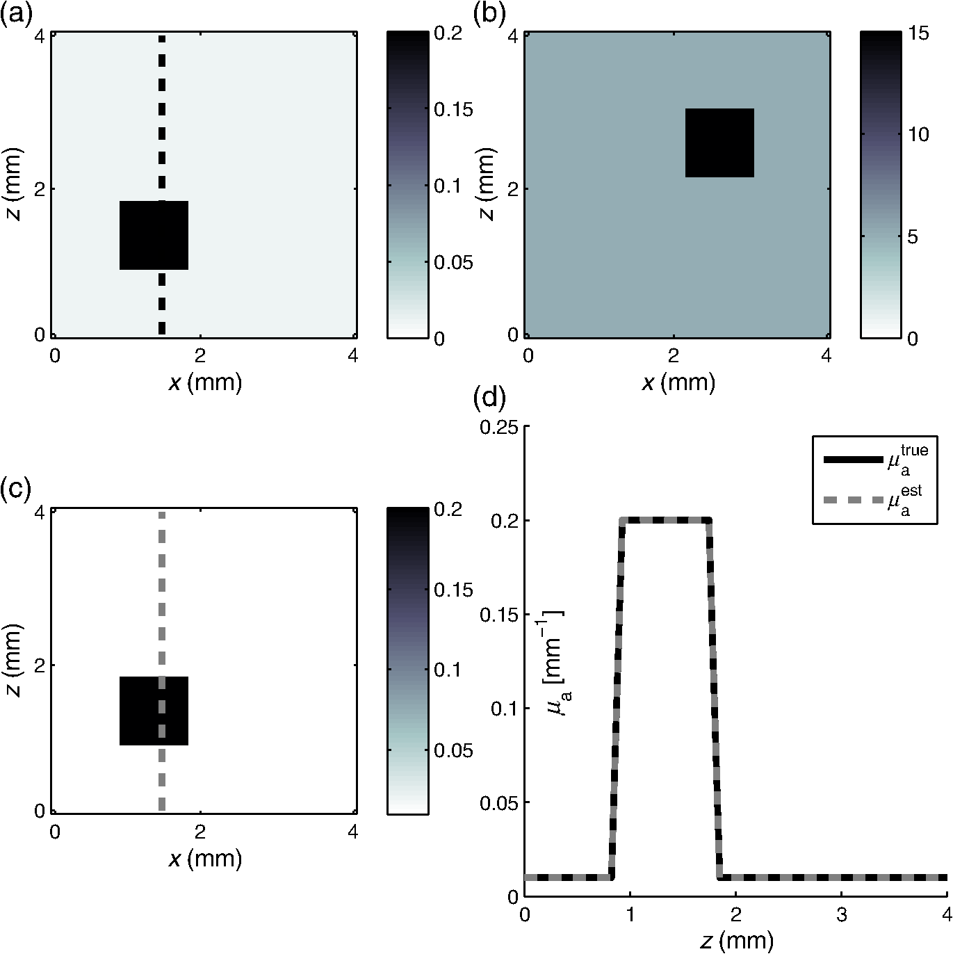$x=1.5\mathrm{mm}$ for all $z$.

Very good agreement between the true and reconstructed absorption coefficient is observed, with a value of the error function after 11 iterations being $2.9\times {10}^{-9}$. The optimization routine was stopped as the change in the error function on the 12th iteration was below the function tolerance of ${10}^{-9}$, indicating convergence. The average error in the estimate of the absorption coefficient ${\mu }_{\mathrm{a}}^{\mathrm{est}}$, computed as $|{\mu }_{\mathrm{a}}^{\text{true}}-{\mu }_{\mathrm{a}}^{\mathrm{est}}|/{\mu }_{\mathrm{a}}^{\text{true}}$, was 0.2% over the entire domain.

6.2.

Inversion for the Scattering Coefficient

Inversions for the scattering coefficient were performed using the same domain as above, shown in Figs. 6(a) and 6(b), with the illumination and number of photons in the forward simulation also being the same. Here, it was assumed that the absorption coefficient was known and the starting estimate of the scattering coefficient was equal to the background value of $5{\mathrm{mm}}^{-1}$.

Fig. 6

(a) True absorption coefficient, (b) true scattering coefficient, (c) reconstructed scattering coefficient after 35 iterations, (d) profiles through true and reconstructed scattering coefficient at $x=2.5\mathrm{mm}$ for all $z$.

Two modifications were necessary to achieve convergence in the optimization for the scattering coefficient. First, a custom GD algorithm was used in which a backtracking line search was implemented. A backtracking line search⁴⁹ starts with a large candidate step length and progressively reduces the step size while checking for a sufficient decrease in the error functional. The sufficient decrease condition is expressed as

Eq. (28)

$$\epsilon ([{\mu }_{\mathrm{a}}^{(i)},{\mu }_{\mathrm{s}}^{(i)}]+{\alpha }^{(i)}{p}^{(i)})\le \epsilon ([{\mu }_{\mathrm{a}}^{(i)},{\mu }_{\mathrm{s}}^{(i)}])+\nu {\alpha }^{(i)}\nabla {\epsilon }^{(i)T}{p}^{(i)},$$

where $\nu$ was chosen to be 0.2 by inspection because this produced rapid convergence. In order to improve efficiency of the line search, step sizes were bounded between $[{10}^5,{10}^9]$; it was found that this range yielded sufficiently large steps to ensure reasonably efficient progress in the minimization. Second, the termination condition in Eq. (27) was relaxed due to the much slower convergence of the scattering coefficient, and instead required a relative change in the error functional of ${10}^{-5}$. This was satisfied after 35 iterations, and is shown in Fig. 6(c) with profiles through the true and reconstructed distributions of ${\mu }_{\mathrm{s}}$ as shown in Fig. 6(d).

It can be seen from Figs. 6(c) and 6(d) that the inversion has partly reconstructed the inclusion in the scattering coefficient. The inability to reconstruct edges of the inclusion in the scattering coefficient is expected, given the diffusive nature of the scattering. However, the discrepancy in ${\mu }_{\mathrm{s}}$ in the inclusion, evident from Fig. 6(d), suggests premature termination of the optimization. This is due to the fact that the gradient with respect to scattering is small and prone to noise in the functional gradients. This low SNR in the gradients has the impact that that search directions in the optimization routine are often suboptimal, which results in little or no progress of the optimization. The progressive reduction in SNR in the gradient means that nondescent steps are likely and can therefore trigger the termination condition.

7.

Discussion and Conclusions

In this paper, an MC model of the RTE was presented. The model computes the radiance in a Fourier basis in 2-D and is straightforward to extend to 3-D using a spherical harmonics basis. The accuracy of the model was demonstrated by comparing the angle-resolved radiance at two positions in the domain to corresponding appropriate analytic solutions.

Sections 5 and 6 presented the application of the RMC algorithm to estimating the absorption and scattering coefficients from simulated PAT images. In Sec. 6.1, it was observed that the absorption coefficient was estimated with an average error of 0.2% over the domain relative to the true value, when the scattering coefficient is known, and in the presence of 0.7% average noise in the data. This is encouraging, particularly because noise is not only present in $H^{\text{meas}}$ but also in the Fourier harmonics computed using the forward and adjoint RMC simulations, which is propagated to the estimates of the functional gradients. Consequently, the search direction in the GD algorithm will always be suboptimal. Furthermore, noise in $H({\mu }_{\mathrm{a}}^{(l)},{\mu }_{\mathrm{s}})$, the estimate of the absorbed energy density at the $l$’th iteration of the line search, will be also be propagated to the error functional, resulting in a nonsmooth search trajectory for the line search because at every point ${\mu }_{\mathrm{a}}^{(l)}$, the error function will be corrupted by some different noise ${\sigma }^{(l)}:\epsilon ({\mu }_{\mathrm{a}}^{(l)},{\mu }_{\mathrm{s}})={\Vert H^{\text{meas}}-H({\mu }_{\mathrm{a}},{\mu }_{\mathrm{s}})(1+{\sigma }^{(l)})\Vert }^2$. In practice, this did not preclude reconstruction of the absorption coefficient since the calculated gradients remained descent directions despite the noise. Furthermore, the error functional in ${\mu }_{\mathrm{a}}$ is sufficiently convex that the addition of some noise does not prevent the linsearch from yielding sufficiently large a step length to allow rapid convergence.

Reconstruction of the scattering coefficent correctly located the scattering perturbation in the simulated image; however, the peak value in the reconstruction was lower than the true value. This is a direct consequence of the fact that the scattering coefficient is related to the absorbed energy distribution only through the optical fluence distribution. Consequently, the SNR in $\frac{\partial \epsilon }{\partial {\mu }_{\mathrm{s}}}$ is typically much less than that for absorption. This causes termination of the algorithm before the peak magnitude of the parameter has been found in the search space.