|
|
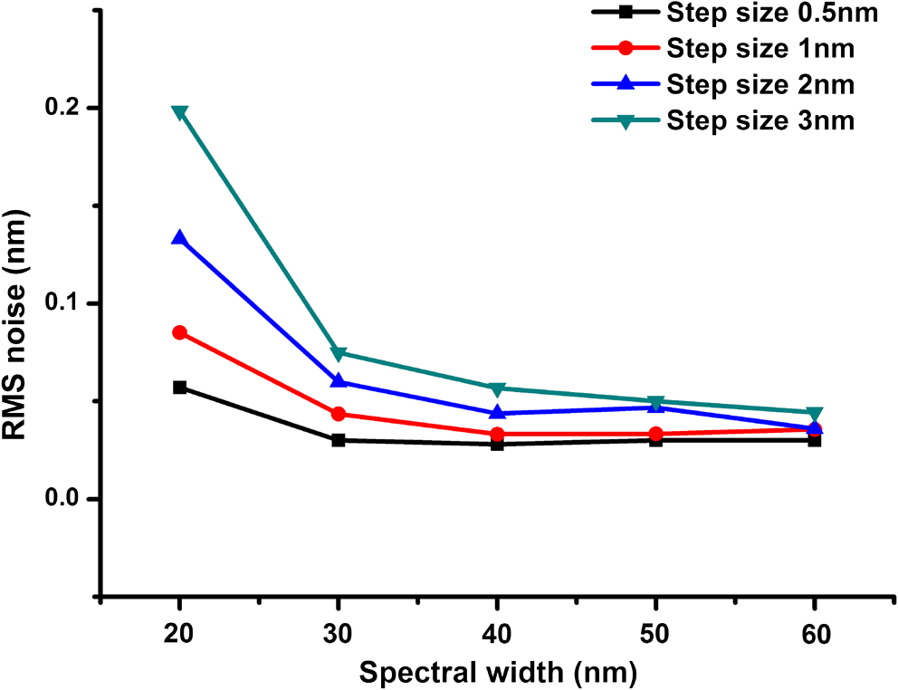
1.IntroductionSurface plasmon resonance (SPR) biosensors, which offer unique real-time and label-free measurement capabilities with high detection sensitivity, have become an important tool for exploring the kinetics of biomolecular interactions and have been widely adopted in detection of chemical and biological analytes.1–4 Moreover, by combining the SPR approach with an imaging system, we can readily achieve high-throughput real-time label-free biosensing in two-dimensional (2-D) microarrays and parallel monitoring of multiple biomolecular interactions.5–9 If the issues related to data-capture speed and detection sensitivity can be adequately resolved, the SPR imaging approach may become a candidate to replace the well-established fluorescence-based microarray technique, which is hobbled by photobleaching and lack of quantitative information. The SPR phenomenon produces a minimum in the reflectivity, called the SPR dip, because the incident p-polarized light resonantly couples with a surface plasma wave at a specific angle or wavelength. The resonant coupling occurs when where is the refractive index (RI) of the prism, is the wavelength of the excitation light, is the real part of a complex dielectric constant of Au, is the angle of incidence, and is the RI of the sample at the metal/dielectric interface.10The position of the SPR dip is very sensitive to changes in the RI of the sample at the metal/dielectric interface. Analyte binding onto the sensor surface will induce a change in the RI at the metal/dielectric interface, thus making it possible to detect the interactions between biological molecules in the vicinity of the metal/dielectric interface through tracking the location of the SPR dip. To accurately determine the position of the SPR dip, three approaches based on intensity, angle, and wavelength interrogations have been developed and widely reported. In the intensity measurement mode, which has the highest imaging speed, the shift of the SPR dip is translated into a change in reflectivity in the linear region of the SPR angular or spectral response curve. This requires both the incidence angle and the wavelength of excitation light to be fixed and optimized for the best possible resolution. However, these requirements severely restrict the choice of operating point and dynamic range over a large sensor surface area and the capacity to simultaneously perform detection of multiple interactions.11 In the angular interrogation mode, the shift of the SPR dip can be monitored by continuous scanning of the SPR angular spectrograph. Compared to the intensity measurement mode, the angular interrogation mode has a wider dynamic range of detection.12 Continuous scanning of the incidence angle by mechanical means in typical angular interrogation-based SPR sensors is slow and usually requires quite complex mechanisms. To overcome these shortcomings, several methods have been reported, including the use of a converging excitation beam,13,14 one-dimensional (1-D) acousto-optical deflector scanner,15 and controlled mirror scanning.16 However, the angular interrogation-based SPR sensor is a compromise in terms of measurement range: the use of a fixed excitation wavelength can offer only the best SPR absorption characteristics within a narrow range of reflective index. The wavelength interrogation-based SPR sensor is much more flexible: the user chooses a range of wavelengths and can select the best spectral window for obtaining the strongest SPR modulation depth.6 Moreover, wavelength interrogation SPR is known to provide a wide dynamic range and the possibility of detection resolution similar to that offered by angle interrogation. In this interrogation mode, a broadband light is used and the SPR spectral profile can be obtained either by scanning the incidence wavelength or by using a spectrometer for analyzing the reflected beam.17–20 If proper data acquisition and analysis schemes have been implemented, the spectrometer-based SPR sensor can provide fast detection of a single sensor site or even 1-D line arrays.21,22 However, this is not a straightforward method for detecting 2-D arrays. Recently, the approach of scanning the incident wavelength has been realized through use of a rotating grating that acts as a fast monochromator.17,23 To realize fast scanning of wavelength for spectral SPR imaging sensors, a nonmechanical liquid crystal tunable filter (LCTF) scanning technique in a fixed wide wavelength range (650 to 1100 nm or 480 to 720 nm) has been developed.24 Large changes in RI may occur when the interaction time is long, analyte concentration levels are high, or the size of the target molecules is large. The spectral SPR sensing design typically sweeps continuously through a wide wavelength range to ensure that the SPR dip never moves out of the range of interest. Moreover, it usually takes for monochromator scanning or 100-ms LCTF scanning to produce a data point on the SPR plot for each wavelength. The measurement time of the SPR dip may not be short enough to achieve real-time monitoring of binding interactions, thereby making it impossible to obtain a true picture of interaction kinetics. Therefore, the issue of achieving a fast scanning speed remains unresolved. To improve measurement speed, a special-fitting algorithm based on using five parameters has been developed for the wavelength interrogation SPR sensors.8,11 The measurement time per SPR dip has been shortened dramatically to 10 s. In this paper, we present a novel fast wavelength-scanning SPR imaging scheme that contains no mechanical moving parts and automatically tracks the movement of the SPR dip using a feedback loop. With the use of an LCTF, the measurement time for an SPR dip is about 4 s, and any spectral range of choice can be scanned at high speed with a good degree of flexibility. To our knowledge, this is the fastest wavelength interrogation SPR imaging sensor ever reported in the literature. The measurement time can be further shortened by a large amount if we also implement the five-parameter fitting algorithms previously reported.11 2.Methods2.1.Experimental SetupFigure 1 shows a schematic of our experimental setup. Light from a 100-W halogen tungsten lamp is coupled to the inverted prism through a multimode optical fiber for SPR excitation. A bandpass filter selects an input wavelength window with a center wavelength of 610 nm and full width at half maximum (FWHM) of 220 nm. The LCTF rapidly scans the output wavelength in a stepwise manner. For our LCTF unit (VariSpec, VIS-10-20-STD), the FWHM, spectral tuning resolution, and response time are, respectively, 10 nm, 0.5 nm, and 50 ms. In our experiments, we chose a wavelength step of 1 nm as this was found to have the lowest level of noise in the final detected signal. While the Kretschmann configuration has been adopted, the SPR cell consists of an equilateral prism made of BK7 glass, a microscope glass slide coated with a 48-nm-thick gold film, and a flow chamber for sample injection. The incident angle can be manually set to an optimized value calculated using Fresnel equations. In the present case, the angle for pure water with an excited wavelength of 660 nm is 72.5 deg. The output light is captured by a 12-bit CCD camera. The A-D card (model number: NI DAQ 6259) generates a triggering signal that synchronizes the operation of the LCTF and CCD camera. An exposure time of is used because of the compromise between camera capture speed and signal-to-noise ratio. In our experiments, it takes 50 ms for the LCTF to switch the wavelength before the CCD starts its exposure cycle. Consequently, the CCD camera records a long series of images taken at different wavelengths within a prescribed spectral range. Figure 2 shows a series of recorded CCD image frames that covers the spectral dip as selected by the LCTF. Each pixel within the CCD image frame provides one wavelength data point within the spectral SPR profile of a small region in the sensor surface. Theoretically, this one-to-one correspondence between the sensor surface and the 2-D CCD imaging pixel arrays may offer massively parallel-biosensing capability. Upon analyzing a series of images, one can build a set of spectral plots that covers all the pixels within the sensor surface. Here, we use a common second order polynomial-fitting algorithm to locate the spectral dip, which corresponds to the resonant wavelength of each pixel. The data analysis procedures are performed in an automatic mode using lab-designed software based on numerical comparison techniques. Fig. 1Schematic of our SPRi system in the Kreschmann configuration. Light from a halogen lamp is collected by a multimode fiber through a set of coupling optics. At the exit end of the fiber, the beam is collimated by a group of lenses and spatially filtered by an aperture before passing through the tunable spectral filter unit and a linear polarizer. The sensor surface is imaged by a CCD camera using two imaging lenses. to : lens; BF: bandpass filter; MF: multimode fiber; DA: diaphragm aperture; LCTF: liquid crystal tunable filter; and : polarizer. 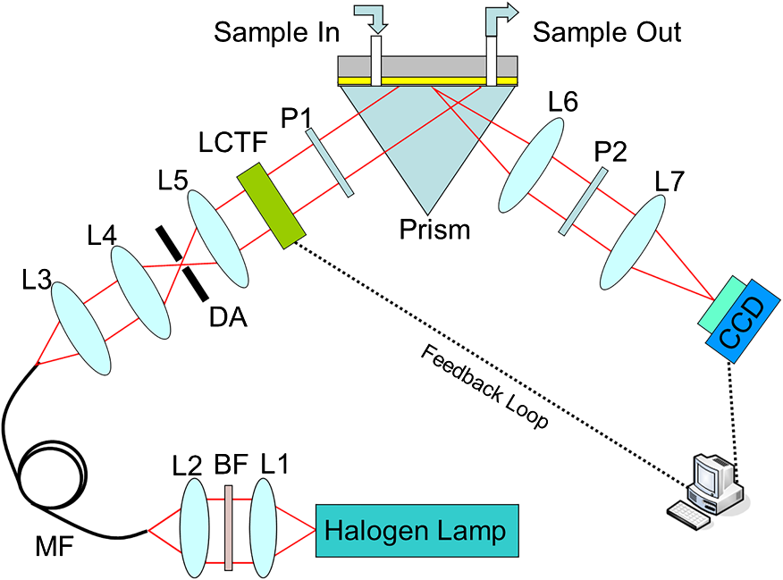 Fig. 2Schematic of the image recording process. Regions marked by A-J represent the sample areas on the chip. First to ’th frame represent a series of images recorded by the CCD camera as we sweep the center wavelength of the LCTF step-by-step. The intensity values of each pixel location taken from the frames constitute one SPR spectral plot, as indicated by the red curve. Therefore, the number of pixels in each image frame corresponds to the number of spectral plots from the system. 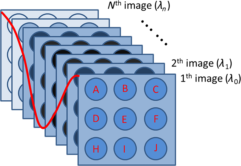 2.2.Feedback LoopThe feedback loop shown in Fig. 1 is designed to automatically track the shift of the SPR dip caused by the binding of target biomolecules. Most importantly, incorporation of this feedback loop drastically reduces the spectral width one needs to sweep before hitting an SPR dip. For example, it takes 80 s to obtain the resonance dip with a traditional stepping monochromator based on a spectral range of 40 nm and a step-size of 1 nm, whereas with the help of a feedback loop, the time required by the present system to find the SPR dip is 4 s. Moreover, an LCTF can scan the incident wavelength across any spectral range according to an optimized strategy with minimal delay. Consequently, the amount of time required to arrive at an SPR resonance data point is significantly shorter. Figure 3 schematically shows how the feedback loop operates. First, an initial SPR spectral profile is obtained by scanning the incident wavelength across a large spectral range to extract the baseline resonant wavelength . Then a spectral range to is chosen. With this, the desired SPR dip with sufficient resolution () (solid red straight line along horizontal axis in which is half the width of the wavelength-scanned range) can be obtained.25 The corresponding partial SPR plot near the SPR dip (red dotted curve) is repeated if the RI of the baseline solution does not change. When a change of RI has taken place, e.g., from to , a new partial SPR plot (solid red curve) is obtained by scanning the incident wavelength from to . Thus, a new resonant wavelength is extracted, then the new scanning spectral range is modified to to (solid green straight line along the horizontal axis). If the RI continues to change from to , the corresponding partial SPR plot (green solid curve) is then updated by scanning the incident wavelength from to . This process will continue until the system has identified the next new resonant wavelength , which will trigger further modification of the scanning range, i.e., from to . In a more general representation, the ’th scanning spectral range, which covers to (solid yellow straight line along the horizontal axis), is generated from the resonant wavelength extracted from the partial SPR plot near the SPR dip obtained in the ’th scanning spectral range of to (solid black straight line along horizontal axis). For a 2-D sensor array, a number of different resonant wavelengths will be obtained from the sensor elements as each of them has been designated to perform a specific sensing task. In such a situation, our system will try to cover the entire range of all the elements by registering the lower and upper limits, i.e., and , of the spectral dip, and the range will become to . Fig. 3Schematic showing the tracking of SPR dip movement based on the feedback loop technique. Here, , and represent a series of RI values at the Au/sample interface when a molecular binding interaction is taking place on the sensor surface. When the RI changes continuously from to , the spectral range to be scanned will also be adjusted automatically from the original spectral range [, ] to [, ] as guided by the feedback loop. This way, only a selected range around the resonance dip will be interrogated at all time, thereby drastically shortening the time to calculate the location of the SPR dip.  3.Results and Discussion3.1.Linearity and Resolution of Surface Plasmon Resonance MeasurementTo estimate the performance of our SPRi system, we measured the RI values of different salt-water mixtures. Salt solutions with a concentration level ranging from 0% to 25% in increments of 5% by volume, which corresponds to a RI ranging from 1.3330 to 1.3793 RIU,26 were prepared. In the experiment, an incident angle of 72.5 deg in the prism was chosen based on the theoretical simulation of the SPR angular dip of water. The scanning spectral range was about 40 nm, and the time for finding the minima of the spectral SPR dip was about 4 s. The array sensor sites, which were uniformly distributed on the chip, were spectrally monitored simultaneously to assess the performance of our system. The step changes of resonant wavelength obtained from different salt concentrations are shown in Fig. 4(a), and the corresponding shifts in spectral SPR dip, as caused by changes in RI, are shown in Fig. 4(b). Based on measurement data obtained in the wavelength range from 600 to 700 nm, the calculated resolution is , and the measured dynamic range of the system is . Here, the conversion from the minimum measurable wavelength shift to the corresponding change in refraction index value is performed with the equation ,26 where is the RI resolution, is the RI change of a bulk medium, is the calculated wavelength shift, and is the estimated wavelength noise. Here, is obtained through averaging 10 measurements of the RMS noise of our system. Fig. 4(a) Shift of SPR dip versus salt concentration in water as detected by sensor sites within the array. (b) Relationship between resonant wavelength of the SPR dip and the shift in RI as detected by the array on the SPR chip. Each data point is obtained by averaging the intensity values of to reduce the effect of noise with no compromise in spatial resolution.  3.2.Application to IgG Interaction MonitoringTo assess the capability of our SPRi system for monitoring biomolecular interactions, we performed real-time monitoring of binding interactions between goat antirabbit IgG and rabbit IgG at different concentration levels. Rabbit IgG was dissolved in the array-spotting buffer at concentrations of 50, 100, 150, and . BSA was chosen as the positive control protein. A array of protein dots was spotted on the SPR chip by hand. Within each column, the three spots had the same solution. The first column on the left was BSA solution; other columns were rabbit IgG solution with concentrations of 250, 150, 100, and , from left to right [see Fig. 5(a)]. The diameter of the spots was about 1 mm, and the distance between the centers of the two adjacent spots was about 2.5 mm. Fig. 5Measurement of goat antirabbit IgG and rabbit IgG antigen–antibody interaction. (a) White light image of the SPR sensor chip, (b–d) real-time wavelength response of antigen–antibody binding interactions, (e–g) SPR shift images of a array obtained after interaction with goat antirabbit IgG solutions of 5, 10, and , respectively. The first column sensor sites, respectively, marked by 11, 21, 31 corresponding to BSA; the second column sites are, respectively, marked by 12, 22, 32, which correspond to rabbit IgG; the third, fourth, and fifth column sites are marked by 13, 23, 33, and 14, 24, 34 and 15, 25, 35, which correspond to 150, 100, and rabbit IgG, respectively. The color of individual SPR plot, i.e., pink, green, blue, red or black, denotes the probe area of , , , , or , respectively.  The IgG interaction procedures were carried out as follows. First, a array chip was attached to the coupling prism using a small drop of RI matching liquid. A piece of molded PDMS was placed over the chip to form a sealed flow cell of (). We designed software to analyze the 15 sensing regions captured by the CCD. A set of 15 spectral SPR plots representing the binding interactions taking place on the spotted sensing regions were generated from the sensor chip. We manually tuned the incidence angle to achieve minimum intensity at the SPR dip for a phosphate buffer saline (PBS) sample. A glycine solution (100 mM, ) was injected for 5 min to regenerate the sensor surface. Next, a buffer solution, PBS , was injected in the flow cell for 3 min with a micropump operating at a speed of to obtain a steady baseline. The initial small scanning range was set at to , in which and were, respectively, the minimum wavelength and maximum wavelength among the resonant wavelengths extracted from all the SPR spectral profiles obtained from the sensing regions. The half width of the scanning spectral range was chosen to achieve the fastest wavelength interrogation and lowest noise. After obtaining a steady baseline for several minutes, the process of capturing the SPR image was automatically executed for one scan to obtain the baseline spectral SPR image, which was produced through extracting the spectral SPR plot of individual sensor sites. Then IgG solutions of 5, 10, and were in turn pumped into the sensor chip. The subsequent antigen–antibody binding interaction taking place on the detection surface was monitored in real time, as shown in Fig. 5. The binding interaction measurement time was typically for each concentration with a constant flow of sample using a syringe pump. After completion of each binding interaction measurement, PBS solution was pumped into the flow chamber for 2 min to ensure adequate buffer washing. To see clearly the shift of the SPR wavelength dip as a function of protein concentration, we arranged the SPR plots into three groups corresponding to the upper, middle, and lower rows of the array. Each group included five members corresponding to four different concentration levels each of IgG and the BSA control sample. As shown in Figs. 5(b)–5(d), the first group showed that the shift of the SPR wavelength dip increases as protein concentration increases in the range from 5 to . Locations on the other two groups on the chip exhibited a similar trend. After completing buffer washing and regeneration steps, the system collects a steady baseline image using data gathered for 3 min, and a reference SPR dip image is produced. Consequently, a reference SPR dip images is available for each IgG concentration. All subsequent SPR dip images obtained while binding interactions were ongoing were analyzed and compared using the first set of reference images and the updated one as the shift of the SPR dip progressed. Figures 5(e)–5(g) show representative images of SPR shift obtained with different protein concentration levels. In the images, the left column of sensor sites shows no change because goat antirabbit IgG does not specifically bind to BSA. In images of other sensor sites, the presence of binding interactions as the SPR dips shift continuously is clearly revealed: the wavelength shift is approximately proportional to the change in concentration of the protein solution. 3.3.Determination of Important ParametersWithin our SPRi technique, interrogation speed is determined by the choice of parameters including step size and total spectral width to be scanned. We analyzed the effects of step size and spectral width on system noise by measuring the variations in SPR dip obtained from pure water. As shown in Fig. 6, for a given step size, system noise decreased and reached a constant level as spectral width increased. Conversely, decreasing the step size decreased the system noise, and the overall interrogation time also increased. For our antigen–antibody interaction experiment, a spectral width of 40 nm and a step size of 1 nm were chosen because they provide optimal performance in terms of noise and interrogation speed under normal curve fitting situations. The salt solution experiment showed that our spectral SPR technique could monitor binding interactions at a rate of about 4 s per data point with an RI resolution and dynamic range similar to that of traditional spectral SPR technique. Spatial resolution is also an important parameter of the SPR imaging system. It primarily defines the density of the final sensor array. We measured the spatial resolution of our SPR imaging system using a standard resolution target. The -axis and -axis resolution limits are 27.8 and , which, respectively, correspond to 6 and 4 pixels of the CCD imaging chip. In our experiments, a area was averaged to improve the signal-to-noise ratio in the process of producing the SPR image. But for all SPR plots, a larger area, i.e., square, was used to obtain the SPR plots for the binding interaction to achieve an optimized signal-to-noise ratio. 4.ConclusionWe have demonstrated a fast wavelength-scanned SPR imaging technique with no mechanical moving parts. By incorporating a feedback loop in the LCTF scanning algorithm, we have drastically reduced measurement time for obtaining spectral SPR dips from a 2-D array. The key function of the feedback loop is to actively follow the movement of the SPR dip while the binding interaction is ongoing so that there is no need to perform wavelength sweeping over an unnecessarily wide spectral range. Compared to the 2-D wavelength-scanning SPR imaging techniques reported in the literature, the proposed spectral SPR sensor has the greatest potential for true real-time label-free monitoring of molecular interactions.18,27,28 Moreover, the detection speed can be further improved, e.g., by increasing the scanning wavelength step, decreasing the scanning wavelength range, or using the five-parameter fitting algorithm.11 Therefore, it is possible for our SPR imaging technology to simultaneously measure the interactions at every spot of a microarray with real-time imaging of the sensor surface. In our experiments, the RI resolution has yet to be better than that of the single wavelength SPR sensor;19,29 this is mainly because the LCTF used in our experiment has a bandpass spectral width of 10 nm. Another source of system noise is not having a precise collimation beam. The angle of the beam divergence decreases the resolution of our SPR system. In the future, we can improve the RI resolution by using a singular value decomposition or minimum hunting method19 or replacing the LCTF with one that offers narrower bandpass width. AcknowledgmentsThis work has been partially supported by the National Major Scientific Research Instruments and Equipment Development Project from National Natural Science Foundation of China (Grant No. 61527827); National Basic Research Program of China (Grant No. 2015CB352005); Guangdong Natural Science Foundation (Grant No. 2014A030312008); Guangdong Province Project (Grant Nos. 2015KGJHZ002 and 2015A020214023); Shenzhen Science and Technology R&D Foundation (Grant No. JCYJ20160422151611496); Collaborative Research Fund (CRF) (Grant No. CUHK1/CRF/12G) from the Hong Kong Research Grants Council, Innovation and Technology Fund (ITF) (Grant No. GHP/014/13SZ) from the Hong Kong Innovation and Technology Commission. ReferencesV. Chabot et al.,
“Biosensing based on surface plasmon resonance and living cells,”
Biosens. Bioelectron., 24
(6), 1667
–1673
(2009). http://dx.doi.org/10.1016/j.bios.2008.08.025 BBIOE4 0956-5663 Google Scholar
J. Homola,
“Surface plasmon resonance sensors for detection of chemical and biological species,”
Chem. Rev., 108
(2), 462
–493
(2008). http://dx.doi.org/10.1021/cr068107d CHREAY 0009-2665 Google Scholar
V. G. Shah et al.,
“Calibration-free concentration analysis of protein biomarkers in human serum using surface plasmon resonance,”
Talanta, 144 801
–808
(2015). http://dx.doi.org/10.1016/j.talanta.2015.06.074 TLNTA2 0039-9140 Google Scholar
C. L. Wong and M. Olivo,
“Surface plasmon resonance imaging sensors: a review,”
Plasmonics, 9
(4), 809
–824
(2014). http://dx.doi.org/10.1007/s11468-013-9662-3 1557-1955 Google Scholar
B. P. Nelson et al.,
“Surface plasmon resonance imaging measurements of DNA and RNA hybridization adsorption onto DNA microarrays,”
Anal. Chem., 73
(22), 1
–7
(2001). http://dx.doi.org/10.1021/ac0010431 Google Scholar
M. Piliarik and J. Homola,
“Surface plasmon resonance (SPR) sensors: approaching their limits?,”
Opt. Express, 17
(19), 16505
–16517
(2009). http://dx.doi.org/10.1364/OE.17.016505 OPEXFF 1094-4087 Google Scholar
S. Scarano et al.,
“Surface plasmon resonance imaging for affinity-based biosensors,”
Biosens. Bioelectron., 25
(5), 957
–966
(2010). http://dx.doi.org/10.1016/j.bios.2009.08.039 BBIOE4 0956-5663 Google Scholar
A. Sereda et al.,
“Compact 5-LEDs illumination system for multi-spectral surface plasmon resonance sensing,”
Sens. Actuators B, 209 208
–211
(2015). http://dx.doi.org/10.1016/j.snb.2014.11.080 Google Scholar
Y. Shao et al.,
“Wavelength-multiplexing phase-sensitive surface plasmon imaging sensor,”
Opt. Lett., 38
(9), 1370
–1372
(2013). http://dx.doi.org/10.1364/OL.38.001370 OPLEDP 0146-9592 Google Scholar
W. Knoll,
“Interfaces and thin films as seen by bound electromagnetic waves,”
Annu. Rev. Phys. Chem., 49 569
–638
(1998). http://dx.doi.org/10.1146/annurev.physchem.49.1.569 ARPLAP 0066-426X Google Scholar
A. Sereda et al.,
“High performance multi-spectral interrogation for surface plasmon resonance imaging sensors,”
Biosens. Bioelectron., 54 175
–180
(2014). http://dx.doi.org/10.1016/j.bios.2013.10.049 BBIOE4 0956-5663 Google Scholar
J. B. Beusink et al.,
“Angle-scanning SPR imaging for detection of biomolecular interactions on microarrays,”
Biosens. Bioelectron., 23
(6), 839
–844
(2008). http://dx.doi.org/10.1016/j.bios.2007.08.025 BBIOE4 0956-5663 Google Scholar
L. Liu et al.,
“Parallel scan spectral surface plasmon resonance imaging,”
Appl. Opt., 47
(30), 5616
–5621
(2008). http://dx.doi.org/10.1364/AO.47.005616 APOPAI 0003-6935 Google Scholar
B. K. Singh and A. C. Hillier,
“Multicolor surface plasmon resonance imaging of ink jet-printed protein microarrays,”
Anal. Chem., 79
(14), 5124
–5132
(2007). http://dx.doi.org/10.1021/ac070755p ANCHAM 0003-2700 Google Scholar
G. D. VanWiggeren et al.,
“A novel optical method providing for high-sensitivity and high-throughput biomolecular interaction analysis,”
Sens. Actuators B, 127
(2), 341
–349
(2007). http://dx.doi.org/10.1016/j.snb.2007.04.032 Google Scholar
N. S. Eum et al.,
“Variable wavelength surface plasmon resonance (SPR) in biosensing,”
Biosystems, 98
(1), 51
–55
(2009). http://dx.doi.org/10.1016/j.biosystems.2009.05.008 BSYMBO 0303-2647 Google Scholar
J. Homola et al.,
“Spectral surface plasmon resonance biosensor for detection of staphylococcal enterotoxin B in milk,”
Int. J. Food Microbiol., 75 61
–69
(2002). http://dx.doi.org/10.1016/S0168-1605(02)00010-7 IJFMDD 0168-1605 Google Scholar
J. S. Yuk et al.,
“Analysis of protein interactions on protein arrays by a wavelength interrogation-based surface plasmon resonance biosensor,”
Proteomics, 4
(11), 3468
–3476
(2004). http://dx.doi.org/10.1002/(ISSN)1615-9861 PROTC 1615-9853 Google Scholar
O. R. Bolduc, L. S. Live and J. F. Masson,
“High-resolution surface plasmon resonance sensors based on a dove prism,”
Talanta, 77
(5), 1680
–1687
(2009). http://dx.doi.org/10.1016/j.talanta.2008.10.006 TLNTA2 0039-9140 Google Scholar
B. Sutapun et al.,
“A multichannel surface plasmon resonance sensor using a new spectral readout system without moving optics,”
Sens. Actuators B, 156 312
–318
(2011). http://dx.doi.org/10.1016/j.snb.2011.04.038 Google Scholar
C. J. Alleyne et al.,
“Analysis of surface plasmon spectro-angular reflectance spectrum: real-time measurement, resolution limits, and applications to biosensing,”
Opt. Lett., 36
(1), 46
–48
(2011). http://dx.doi.org/10.1364/OL.36.000046 OPLEDP 0146-9592 Google Scholar
F. Bardin et al.,
“Surface plasmon resonance spectro-imaging sensor and associated data processing for biomolecular surface interaction characterization,”
Proc. SPIE, 6450 64500N
(2007). http://dx.doi.org/10.1117/12.700882 PSISDG 0277-786X Google Scholar
S. Otsuki and M. Ishikawa,
“Wavelength-scanning surface plasmon resonance imaging for label-free multiplexed protein microarray assay,”
Biosens. Bioelectron., 26
(1), 202
–206
(2010). http://dx.doi.org/10.1016/j.bios.2010.06.017 BBIOE4 0956-5663 Google Scholar
J. A. Ruemmele et al.,
“A localized surface plasmon resonance imaging instrument for multiplexed biosensing,”
Anal. Chem., 85
(9), 4560
–4566
(2013). http://dx.doi.org/10.1021/ac400192f ANCHAM 0003-2700 Google Scholar
M. Palumbo et al.,
“A single chip multi-channel surface plasmon resonance imaging system,”
Sens. Actuators B Chem., 90 264
–270
(2003). http://dx.doi.org/10.1016/S0925-4005(03)00041-8 Google Scholar
S. P. Ng et al.,
“White-light spectral interferometry for surface plasmon resonance sensing applications,”
Opt. Express, 19
(5), 4521
–4527
(2011). http://dx.doi.org/10.1364/OE.19.004521 OPEXFF 1094-4087 Google Scholar
F. Bardin et al.,
“Surface plasmon resonance spectro-imaging sensor for biomolecular surface interaction characterization,”
Biosens. Bioelectron., 24
(7), 2100
–2105
(2009). http://dx.doi.org/10.1016/j.bios.2008.10.023 BBIOE4 0956-5663 Google Scholar
L. Liu et al.,
“A two-dimensional polarization interferometry based parallel scan angular surface plasmon resonance biosensor,”
Rev. Sci. Instrum., 82
(2), 023109
(2011). http://dx.doi.org/10.1063/1.3553028 Google Scholar
A. Abbas, M. J. Linman and Q. Cheng,
“New trends in instrumental design for surface plasmon resonance-based biosensors,”
Biosens. Bioelectron., 26
(5), 1815
–1824
(2011). http://dx.doi.org/10.1016/j.bios.2010.09.030 BBIOE4 0956-5663 Google Scholar
BiographyKaiqiang Chen graduated with a BEng degree from Huazhong University of Science and Technology Wenhua College. Currently, he is an MEng student in the College of Optoelectronics Engineering, Shenzhen University. His research mainly involves the development of surface resonance sensors for biomedical applications. Youjun Zeng was awarded a BSc degree from Changchun University of Science and Technology. He is currently an MEng student in the College of Optoelectronics Engineering, Shenzhen University. His research focuses on surface resonance imaging technique. Lei Wang was awarded a BSc degree from Changchun University of Science and Technology. He is currently an MEng student in the College of Optoelectronics Engineering, Shenzhen University. His research focuses on surface resonance imaging technique. Dayong Gu earned his MD degree from Third Military Medical University. Currently, he is a senior researcher at Central Laboratory of Health Quarantine, Shenzhen International Travel Health Care Center, Shenzhen Entry-Exit Inspection and Quarantine Bureau, China. His research interests include microbial molecular diagnostic techniques and optical biosensors. Jianan He received his PhD in the College of Engineering at Peking University in 2011. He is an associate professor of Shenzhen Entry-Exit inspection and Quarantine Bureau. He was a postdoctoral fellow at Peking University from 2011 to 2013. His research focuses on biosensors, particularly development of chemical surface for biomedical and infectious disease diagnostics applications. Shu-Yuen Wu received his BSc and MPhil degrees in applied physics from The City University of Hong Kong. He continued to study electronic engineering and received his PhD at The Chinese University of Hong Kong. He is working on biosensing systems related to surface plasmon resonance, laboratory on a disk (LOAD) system, nanoparticles, and nanoislands. Ho-Pui Ho received his BEng and PhD degrees in electrical and electronic engineering from the University of Nottingham. His academic interests include nanosized semiconductor materials for photonic and sensor applications, optical instrumentation, surface plasmon resonance biosensors, lab-on-a-chip, and biophotonics. He has published over 270 peer-reviewed articles, and holds 15 Chinese and 5 US patents. He is a fellow of SPIE and HKIE, and a senior member of IEEE. Xuejin Li received his PhD in physical electronics from Tianjin University in 2005. He developed his interest in fiber optic sensor technologies, their principles and applications. He now works as the director of the Shenzhen Key Laboratory of Sensor Technology and Shenzhen Engineering Laboratory for Optical Fiber Sensors and Networks, Shenzhen University. He was awarded the Outstanding Scholar of Shenzhen University in 2013. He has published over 80 papers. Junle Qu received his PhD in 1998 from Xi’an Institute of Optics and Precision Mechanics, Chinese Academy of Sciences. He is currently a professor of optical engineering at Shenzhen University. His research interests include nonlinear optical microscopy, fluorescence lifetime imaging and super-resolution optical imaging. He published over 120 papers in peer-reviewed journals and holds 20 patents. He is a senior member of SPIE and the Chinese Optical Society (COS), and the director of COS Biomedical Photonics Committee. Bruce Zhi Gao received his BS and MS degrees, respectively, in optoelectronics in 1985 and applied laser physics in 1988, both from Tianjin University, China. He received his PhD in biomedical engineering from the University of Miami in 1999, then followed a 3-year postdoctoral training in cell and tissue engineering at the University of Minnesota. He is currently a professor and the director of the biophotonics lab in the Department of Bioengineering at Clemson University. Yonghong Shao obtained his PhD in optics from Changchun Institute of Optics, Fine Mechanics, and Physics, Chinese Academy of Science, China. Currently, he is a professor at Key Laboratory of Optoelectronic Devices and Systems of Ministry of Education and Guangdong Province, Shenzhen University. His research interests involve surface plasmon resonance sensors, multiphoton fluorescence microscopy and confocal endoscopy. He has published over 40 papers and 17 Chinese patents. |