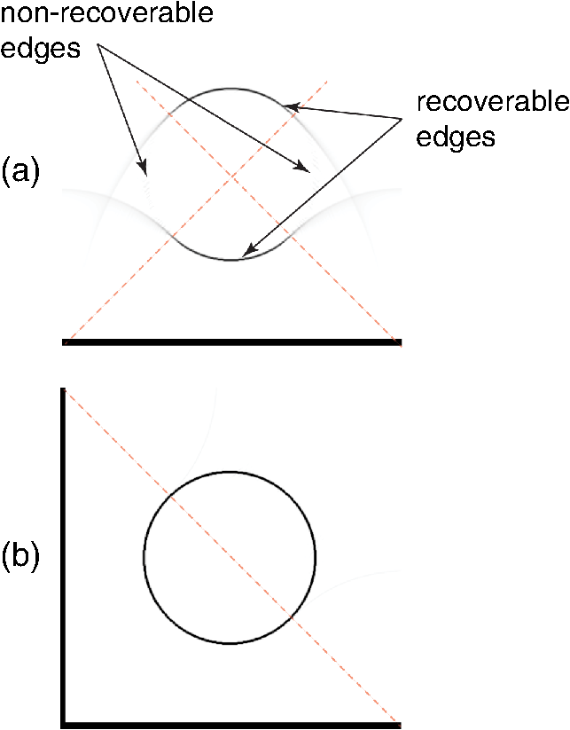2.1.

L-shaped Fabry–Pérot Sensor

FP sensors consist of mirrors separated by a polymer spacer layer.² The FP sensor mirrors are dichroic and designed to allow wavelengths in the 600 to 1200-nm range to be transmitted while reflecting the longer wavelengths used for interrogation (1500 to 1600 nm). This allows the photoacoustic excitation light to be introduced through the sensor to achieve backward mode illumination. The FP sensors were interrogated by a focused wavelength tunable laser beam, which was scanned to different spatial locations across the sensor to synthesize array measurements. At each location, the wavelength of the interrogation beam is tuned to the maximum slope of the interferometer transfer function (ITF), measured prior to acquisition. When an acoustic wave passes through the FP sensor, it modulates the spacer thickness, and, through the ITF, the power of the reflected light from the sensor changes proportionately.² The slope of the ITF determines the sensitivity of the sensor at each location. To correct for variation in sensitivity from location to location, the data from each sensor are normalized to the slope of the ITF.

Previous work on FP sensors has concentrated on planar arrays.² In this work, an L-shaped sensor was developed, consisting of two orthogonal, planar FP sensor arrays. Due to practical fabrication considerations, planar FP sensors typically exhibit an inactive region around their outer edge, where the sensor is sealed to the mounting point of the water tank [Fig. 3(a)]. However, when used in conjunction with a second, orthogonal, sensor, the inactive regions prevent the detection of the acoustic field in a strip close to the vertex between the sensors, which can have a detrimental effect on the reconstructed image.²⁰ To overcome this, new sensors were produced with part of the substrate removed to reduce the insensitive area between the active regions [Fig. 3(b)]. To seal these sensors, a custom tray was produced. The sensors produced for this system have a spacer thickness of $22\mu \mathrm{m}$, giving a nominal $-3\mathrm{dB}$ bandwidth of 39 MHz.

Fig. 3

Sensor fabrication. (a) An L-shaped sensor with an inactive region around the edge of each planar part, leading to a region of insensitivity in the sensor’s central valley. (b) A modified sensor with no central insensitive region.

2.2.

Interrogation System

Two identical optical systems were used to interrogate the orthogonal sensors. Each interrogation system consisted of a custom $x\text{-}y$ scanner² that scanned the position of a focused beam from a wavelength tunable laser (1500 to 1610 nm, Yenista Optics Tunics- T100S-HP) across the FP. Two interrogation lasers were used, one for each sensor plane, and the light reflected from each sensor was detected using identical custom photodiodes. Each photodiode consisted of an InGas photodiode with a transimpedance amplifier with a nominal bandwidth of 100 MHz and AC and DC coupled outputs. The DC-coupled outputs from each photodiode were connected to separate $250\mathrm{KS}/\mathrm{s}$ 16-bit analogue-to-digital (A/D) cards (NI PCIe-6323) in the PC to record the transfer functions of the sensors, as part of the wavelength-biasing scheme. The AC-coupled outputs from each photodiode were captured on separate channels of a single digitizer card (125 MHz bandwidth, NI PCI-5114) to record the acoustic signals.

The sensors were rigidly connected by the water-tight tray and could not be moved relative to each other. To align the scanners to their respective sensors simultaneously, therefore, the positions of the scanners, rather than the sensors, had to be adjusted. To ensure that each scanner was held mechanically stable relative to its sensor, they were mounted on custom mechanical armatures that allowed each system to be positioned through six degrees of freedom relative to the sensors.

2.3.

Photoacoustic Excitation Source

The excitation source for all the phantom studies was a Q-switched Nd:YAG laser (Big Sky, Ultra) operating at 1064 nm (8-ns pulse length). For the mouse imaging in Sec. 4.2, to ensure optimum SNR, two Nd-YAG pumped optical parametric oscillators (OPO’s), a GWU VisIR pumped by a Spectra-Physics Quanta Ray LAB170 and an Innolas Spitlight 600 with pulse widths of 8 and 6 ns, respectively, were used to generate the photoacoustic signals. The two OPOs had pulse energies of 20 and 12 mJ, and a pulse repetition rate of 10 Hz. The output of each OPO source was coupled into the sample in backward mode, through each sensor, via a dichroic mirror, as shown in Fig. 2(a). The beams were expanded so the fluence on the tissue surface was about $9\mathrm{mJ}/{\mathrm{cm}}^2$, well below the maximum permissible exposure. The OPOs were triggered such that the pulses they emitted were synchronized to within $\pm 2\mathrm{ns}$ of each other using a combination of custom electronics and an Agilent 33522A signal generator with a repetition rate of 10 Hz. Both OPOs were configured to a wavelength of 755 nm.

2.4.

Registration Procedure

To locate the relative positions of the detection points on the two sensor planes in a unified coordinate system, a registation procedure was developed. A registration phantom was produced consisting of three black polymer strands mounted to a custom acrylic mount [Fig. 4(a)]. The phantom was imaged over a region of $10\mathrm{mm}\times 15\mathrm{mm}$ by each sensor. Care was taken to ensure the registration phantom was thermally stable during the registration procedure. A step size of 50 or $100\mu \mathrm{m}$ was used. The data from each sensor were then reconstructed separately using time reversal.^26,27 The sound speed was selected automatically.²⁸ Thresholding was used to generate point clouds from each. A registration algorithm²⁹ was then applied to these point clouds to obtain the rigid transformation between their local, on-plane, coordinate systems. In Fig. 4(c), an example of the point cloud from each sensor aligned to a common coordinate system is shown; the circles relate to data from sensor X and the crosses from sensor Y [see Fig. 2(b)]. The relative positions of the detection points on sensors X and Y are also shown in Fig. 4(c). The accuracy of this alignment procedure was of the order of a pixel width (100 or $50\mu \mathrm{m}$ dependent on the acquisition step size).

Fig. 4

(a) The phantom, consisting of three black $17\text{-}\mu \mathrm{m}$ polymer strands on a transparent acrylic mount, used for registration. (b) The phantom with multiple parallel polymer strands used in the resolution measurements (Sec. 3). (c) The positions of the sensor detection points (triangles) and the registration phantom postregistration. The registration phantom is shown as seen by sensor X (circles) and sensor Y (crosses), showing they are well-registered. (The number of sensor points was downsampled for visual clarity.)

2.5.

Image Reconstruction

To reconstruct an image using the L-shaped sensor, an iterative time reversal technique was employed,^30,31 incorporating the dual constraints of positive initial pressure and zero initial particle velocity. This technique effectively adds successive terms in a Neumann series and will converge on the correct solution given sufficient data. The sequence of images $p_0^{(m)}$ was given by Eq. (1):

Although there was strictly no “visible region” in which an exact image can be obtained due to the absence of a third orthogonal detection plane, the artifacts in the planes orthogonal to the L-shaped sensor were reduced considerably. It is important to note that the image resulting from the iterative reconstruction will not be just the sum of the two images obtained using the planar sensors. Instead, it will have fewer artifacts due to the L-shaped sensor’s improved visibility and the suppression of the artifacts in the iterative reconstruction due to the non-negativity and zero initial particle velocity constraints (note there is no exact noniterative reconstruction for this geometry). The numerical model used for both the forward and time reversal operations was a k-space pseudospectral time-domain propagation model, k-wave.^32,33 When using only a single planar sensor, for comparison, a time reversal technique^26,27 was used to reconstruct the image.

3.1.

Numerical Simulations

Several factors affect the resolution of the images obtained using a FP sensor, including the spatial sampling interval, the effective element size, the bandwidth of the sensor (primarily related to the spacer thickness), and the detection aperture size and configuration.² The calculated effective element diameter in the case of these sensors is $\sim 60\mu \mathrm{m}$, based on a sensor spacer thickness of $22\mu \mathrm{m}$ and a Gaussian waist diameter of $49\mu \mathrm{m}$ at an acoustic frequency of 25 MHz.³⁴ To investigate the spatial resolution of the L-shaped sensor in comparison to a planar sensor, several simulations were carried out using k-wave.^32,33 A numerical phantom consisting of absorbing lines parallel to the $z$-axis was created. As the absorbing lines were parallel to the sensor, a 2-D simulation was sufficient to generate the predicted acoustic fields due to the translational invariance in the $z$-direction. A 2-D domain of $18\mathrm{mm}\times 18\mathrm{mm}$ was discretized into a grid with a step size of $20\mu \mathrm{m}$; a time step of 4 ns was used. The sound speed of the medium was set to the value for water, $1480{\mathrm{ms}}^{-1}$.³⁵ Sensor arrays consisting of elements with a width of $60\mu {\mathrm{m}}^2$ were placed on two sides of the domain. The time series were filtered to be representative of the frequency response of a sensor with a $22\text{-}\mu \mathrm{m}$ spacer.^36,37 The 2-D simulation was then extended into the $z$-dimension by including multiple copies of the time series along the $z$-axis to simulate the effect of a detection array with width 0.4 mm in the $z$-direction. This 3-D dataset was then used to reconstruct an image using iterative time reversal (10 iterations). The central slice through the reconstructed image was extracted, and profiles in the $x$ and $y$-direction were taken through each point. A Gaussian was fitted to the profile, and the full-width half-maximum (FWHM) of this Gaussian was determined using the relationship:

3.2.

Experimental Results

The point spread functions (PSFs) for the planar and L-shaped arrays were measured and compared to the simulation results. A phantom with a cross-section significantly smaller than the expected lateral resolution is required to measure the PSF. Based on previous measurements using a $22\text{-}\mu \mathrm{m}$-thick planar FP sensor,² which demonstrated a lateral resolution of $40\mu \mathrm{m}$, absorbing polymer strands with a diameter of $17\mu \mathrm{m}$ were judged to meet this criterion. A target was constructed consisting of 32 of these polymer strands mounted within a custom polymer mount designed to avoid blocking the acoustic path between the sensors and the strands [Fig. 4(b)]. The strands were dyed using India ink for contrast.

The phantom was imaged photoacoustically over an area of $18\mathrm{mm}\times 18\mathrm{mm}\times 0.5\mathrm{mm}$ with a step size of $20\mu \mathrm{m}$. Each dataset was then reconstructed as outlined in Sec. 2.5. Slices of the 3-D images were taken. Figures 5(a) and 5(c) show a region of these images containing a single strand for the planar and L-shaped sensors, respectively. To obtain the resolutions in the $x$ and $y$ directions, a two term Gaussian model was fitted to the maximum intensity projections of these images (in the $x$ and $y$ directions, respectively), and the FWHM of the narrower Gaussian was taken as the resolution. This is shown for the $x$-resolution (horizontal resolution) in Figs. 5(b) and 5(d) for the planar and L-shaped sensors, respectively. Maximum intensity projections of the images, rather than profiles along a line through the centre of the feature, were used to ameliorate the noncircular shape of the PSFs and give profiles more suitable for the Gaussian fitting.

Fig. 5

Spatial resolution measurement method. (a) Cross-sectional image of one absorbing strand obtained with a planar sensor. (b) Vertical maximum intensity projection of image (a), giving the horizontal profile shown by crosses to which a two-term Gaussian was fitted (solid line) and the FWHM of the narrower Gaussian (dashed line) was taken as the resolution. (c) Reconstruction of the same feature as in (a) obtained with the L-shaped sensor. (d) The equivalent to (c) for the L-shaped sensor.

Figure 6 shows the $x$- and $y$-resolutions for the planar and L-shaped sensors, from both the simulation (grayscale map) and the experiment (points with values in microns below). Figure 6(a) shows the resolution in the $x$-direction using data from a planar sensor (sensor X). In this case, the resolution decreases with increasing distance from the sensor, largely due to the limited detection aperture. Figure 6(c) shows the resolution in the $y$-direction using data from planar sensor X. It is notable that it is considerably better than the $x$-direction resolution for the same sensor. This is due, in part, to the fact that the data were recorded with a higher temporal sampling than the equivalent spatial sampling. As the vertical wavenumber components of the initial pressure distribution (those in the $y$ direction in this case) are encoded onto the temporal waveforms, a higher temporal bandwidth results in improved spatial resolution in the $y$-direction.

Fig. 6

Spatial resolution. Simulated results shown in grayscale, and dots with values below show the experimental values in $\mu \mathrm{m}$. Domain size $18\mathrm{mm}\times 18\mathrm{mm}$. Resolution in the $x$-direction when using (a) planar sensor X and (b) the L-shaped sensor. Resolution in the $y$-direction when using (c) planar sensor X and (d) the L-shaped sensor.

Figure 6(b) shows the $x$-resolution for the L-shaped sensor [compare Fig. 6(a)]. In this case, a more uniform resolution was achieved throughout the field of view, with higher resolution everywhere compared to the planar sensor. However, there is, in general, an increase in the $x$-resolution close to sensor Y. This is another manifestation of the higher temporal than spatial sampling. In this case, the temporal sampling of sensor Y is higher than the spatial sampling of sensor X, so the $x$-resolution improves closer to sensor Y. [And vice-versa: the $y$-resolution improves closer to sensor X, Fig. 6(d).] This effect was also observed by Paltauf et al.⁹ and Li et al.²³

Figure 6(d) shows the $y$-resolution for the L-shaped sensor. Considering the symmetry of the L-shaped sensor, it is no surprise that the simulated resolution map in Fig. 6(d) is the same as Fig. 6(b), flipped about the $x-y$ axis. The variance in the experimental data makes this harder to discern, but in general a similar pattern is observed.

Table 1 shows a comparison between the mean values of resolution for the simulation and experimental data. The measured data matches well to the simulation for the L-shaped sensor, although the experimental values are slightly higher than the simulation due to noise in the experimental data. The reduction in the lateral resolution is also significant: the average $x$-resolution in the field of view of the L-shaped sensor was $60\mu \mathrm{m}$, whereas the average $x$-resolution for the planar sensor in the same region was $99\mu \mathrm{m}$. Closer to the planar sensor, the resolution achieved more closely matches that of the L-shaped sensor. Finally, the improved isotropy in the resolution of the L-shaped sensor compared to the planer sensor is clear from these averages: the $x$- and $y$-resolutions for the L-shaped sensor are comparable, but for the planar sensor, they differ by more than a factor of 2. While on average, the resolutions are similar in both directions, at many points in the image, some anisotropy will remain due to the difference in the spatial and temporal sampling rates.

Table 1

Comparison of mean values of resolution, in both x and y directions, for the simulated and experimental data for both sensor geometries.

4.1.

Leaf Phantom

A skeletal leaf was used as a phantom to demonstrate the ability of the system to provide improved view of features oriented in both the $x$ and $y$ directions. The contrast was enhanced by submerging the leaf in India ink for an hour, after which it was removed and allowed to dry for 24 h. The slightly curved leaf skeleton was positioned approximately perpendicular to both sensors and orientated so that there were veins visible to one sensor while not being visible to the other sensor and vice-versa. The leaf phantom, shown in Fig. 7(a), was scanned over an area of $20\mathrm{mm}\times 10\mathrm{mm}$ on each sensor, with a step size of $100\mu \mathrm{m}$, giving an overall imaged volume of $26\times 26\times 10\mathrm{mm}$ (including the gap region between the sensors, see Fig. 3). Reconstructions were performed on an upscaled grid of $50\mu \mathrm{m}$. Figures 7(b) and 7(c) show the reconstructions for each independent planar sensor. The data from each sensor were separately reconstructed using time reversal.^26,27 Clearly, in both cases, those veins that were perpendicular to the sensor were not recovered, but the veins that ran parallel were recovered. The data from the L-shaped sensor were reconstructed using 10 iterations of an iterative time reversal reconstruction,^30,31 as described in Sec. 2.5. Figure 7(d) shows the resulting image, and it is evident that in this case, the majority of the features in both orientations are recovered well.

Fig. 7

Photoacoustic images of a leaf phantom. (a) Photograph of leaf phantom. (b) Maximum intensity projection (MIP) of image obtained using a planar sensor along lower side. (c) MIP of image obtained using a planar sensor to the left of the domain. (d) MIP of the image obtained using the L-shaped sensor. Inset in (b), (c) and (d): zoomed image sections.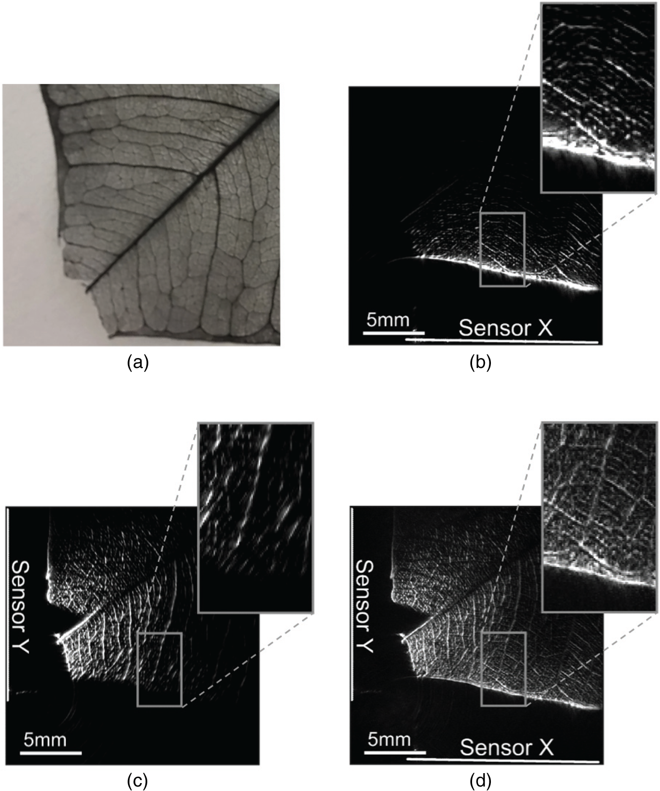

4.2.

Mouse Imaging

A mouse, postmortem, was placed into the scanner and imaged over a $13.4\times 14\times 16\mathrm{mm}$ volume around the head region with a step size of $100\mu \mathrm{m}$. The mouse was orientated such that the top of the head was pointing toward the joint between the sensor planes. All experiments were performed in accordance with the UK Home Office Animals Scientific Procedures Act (1986). Sufficient deionized water was used to couple just the part of the mouse being imaged. Excitation light ($\lambda =755\mathrm{nm}$) was introduced into the volume in backward mode through both sensors. Three reconstructions were completed, one for each planar sensor independently and another for the L-shaped sensor. Figure 8 shows maximum intensity projections of the same region in three different directions: $x$-projection (looking through sensor Y), $y$-projection (looking through sensor X), and $z$-projection (looking along between the sensors). For each view, three images are given, corresponding to that formed using data from sensor X only, sensor Y only, and both sensors X and Y, i.e., the L-shaped sensor. As with the leaf phantom, the reconstructions from the planar sensors show structures that run parallel to the sensor while suppressing perpendicular structures. The L-shaped sensor gives a more complete reconstruction. Several features of the murine cerebral vasculature are visible in this image, including the superior sagittal sinus, transverse sinus, and the inferior cerebral vein, as well as the retinal vasculature of the eyes.

Fig. 8

Ex-vivo images of mouse head. Row (a) MIPs along the $x$-direction obtained using sensor X, sensor Y, and the L-shaped sensor, respectively. Row (b) MIPs along the $y$-direction obtained using sensor X, sensor Y, and the L-shaped sensor, respectively. Row (c) MIPs along the $z$-direction obtained using sensor X, sensor Y, and the L-shaped sensor, respectively. The schematic (d) shows the respective orientation of the mouse, sensor, and coordinate system. Major vessels and structures in the mouse head are clearly visible, including the transverse sinus (TS), superior sagittal sinus (SSS), inferior cerebral vein (ICV), and the retina of the eyes (E).

For a second demonstration, the abdominal region of the mouse was imaged using each planar sensor independently and the L-shaped sensor. The mouse was positioned such that one side of the abdomen sat between the two sensors. Figure 9 shows three maximum intensity projections in the $z$-direction (looking along between the sensor planes) of the same region. Figures 9(a) and 9(b) use data from a planar sensor X and Y, respectively. Different features—those parallel to the sensor used—are visible in each. When the L-shaped sensor is used, a clear improvement in the sharpness of the structures at depth can be seen. The boundary of the kidney, arrowed in Fig. 9(c), and its internal structure are particularly clear, with the interior vasculature more completely resolved. The spleen is also well recovered, labeled S [Fig. 9(c)]. The surface and deep vasculature are also imaged more clearly in this case, compared to either planar sensor alone.

Fig. 9

Ex-vivo images of mouse abdomen. (a) MIP along the z-direction, obtained using the data from sensor X. (b) MIP obtained using the data from sensor Y. (c) MIP obtained using the L-shaped sensor (i.e., data from sensors X and Y). Both the kidney (arrowed) and spleen (S) can be clearly seen.

Figure 10 shows slices through the images of the same region of the abdomen obtained by (a) the planar and (b) L-shaped sensors, respectively. First, it is clear that the shape of the kidney is distorted in Fig. 10(a) compared to Fig. 10(b). Second, comparing the structure circled in both images, it is clear from Fig. 10(b) but not from Fig. 10(a) that this is a vessel running in the z-direction (into the image). The reduction in artifacts demonstrates that images produced using the L-shaped sensor are not just the sum of two images from the planar sensors. This exemplifies the type of image improvement that an L-shaped sensor can provide over a planar sensor and shows that it can facilitate higher fidelity images, especially of deeper lying anatomical structures.

Fig. 10

Slices through ex-vivo kidney image. (a) A slice through the image whose MIP is shown in Fig. 9(a), obtained using planar sensor X. (b) A slice through the image whose MIP is shown in Fig. 9(c), obtained using the L-shaped sensor. The circled feature and the improved recovery of the kidney shape demonstrate the reduction in artifacts that can be achieved using the L-shaped sensor.