Diffuse shear wave imaging: toward passive elastography using low-frame rate spectral-domain optical coherence tomography

Thu-Mai Nguyen; Ali Zorgani; Maxime Lescanne; Claude Boccara; Mathias Fink; Stefan Catheline

doi:10.1117/1.JBO.21.12.126013

21 December 2016 Diffuse shear wave imaging: toward passive elastography using low-frame rate spectral-domain optical coherence tomography

Thu-Mai Nguyen, Ali Zorgani, Maxime Lescanne, Claude Boccara, Mathias Fink, Stefan Catheline

Author Affiliations +

Journal of Biomedical Optics, Vol. 21, Issue 12, 126013 (December 2016). https://doi.org/10.1117/1.JBO.21.12.126013

Abstract

Optical coherence tomography (OCT) can map the stiffness of biological tissue by imaging mechanical perturbations (shear waves) propagating in the tissue. Most shear wave elastography (SWE) techniques rely on active shear sources to generate controlled displacements that are tracked at ultrafast imaging rates. Here, we propose a noise-correlation approach to retrieve stiffness information from the imaging of diffuse displacement fields using low-frame rate spectral-domain OCT. We demonstrated the method on tissue-mimicking phantoms and validated the results by comparison with classic ultrafast SWE. Then we investigated the in vivo feasibility on the eye of an anesthetized rat by applying noise correlation to naturally occurring displacements. The results suggest a great potential for passive elastography based on the detection of natural pulsatile motions using conventional spectral-domain OCT systems. This would facilitate the transfer of OCT-elastography to clinical practice, in particular, in ophthalmology or dermatology.

1. Introduction

Dynamic shear wave elastography (SWE) consists of deducing the viscoelastic properties of soft tissue from the characteristics of mechanical perturbations propagating in the tissue. In soft, incompressible tissue, the elastic behavior is dominated by the shear modulus $μ$ and the stiffness can be characterized by $E = 3 μ = 3 ρ c_{shear}^{2}$ , where $E$ is the Young’s modulus, $ρ$ is the tissue density, and $c_{shear}$ is the speed of a shear wave propagating across the tissue.¹ One of the most common SWE techniques, introduced by Sarvazyan et al.,² consists of actively launching a micron-scale shear wave in the tissue and tracking its propagation to measure its speed. This technique, first implemented using magnetic resonance imaging or ultrasound imaging in the late 1990s,³^–⁵ has been recently extended to optical coherence tomography (OCT) for elastography at micron-scale resolution with medical applications in ophthalmology and dermatology. OCT can be used for phase-sensitive speckle-tracking of displacements within tissue⁶^,⁷ and current technological developments enable to reach frame rates between tens and hundreds of kilohertz.⁸^,⁹ The OCT setups are combined with external active shear sources, such as mechanical actuators,¹⁰ air-puffs,¹¹^–¹³ ultrasonic radiation force,¹⁴^–¹⁶ or a photoacoustic effect.¹⁷^,¹⁸ Although efficient, some of these shear sources may present disadvantages for clinical implementation in ophthalmology: mechanical actuators need to be placed in contact with the tissue; ultrasonic radiation force and photoacoustic effects expose the tissue to relatively high ultrasound pressures or high laser fluences; air-puffs have only been demonstrated on superficial tissues so far. In ophthalmology, in particular, it can be challenging to generate displacements in deeper ocular tissues such as the crystalline lens or the retina.

Passive elastography methods have emerged in the past few years, inspired from techniques based on ambient seismic noise correlation developed in several fields such as helioseismology,¹⁹^,²⁰ oceanography,²¹^,²² and ultrasonics.²³ The correlation of a noise-like signal allows the extraction of information from a broadband and multiply scattered signal. It consists of retrieving wave speed maps from permanent ambient seismic noise. In the human body, heart beats and muscular activities create a permanent physiological noise. Naturally induced shear waves have already been used to qualitatively assess the elastic parameters.²⁴^,²⁵ The ability of a noise-correlation technique to passively retrieve the elastic parameter in vivo has been shown in Refs. 26 and 27. From a physics point of view, it has been demonstrated that time reversal (TR) of a diffuse wave field is equivalent to correlation methods.²⁸^,²⁹ This equivalence will be frequently used in this study. The possibility to use TR-based techniques with a low-frame rate ultrasound scanner has been demonstrated, both in a calibrated phantom and in healthy living tissue.³⁰ With low-frame rate imaging systems, because of the lack of temporal information, only shear wavelength maps instead of shear wave speed maps can be provided.

Here, we propose to implement a TR-based approach for SWE using standard spectral-domain OCT (SD-OCT): SD-OCT is used to image a diffuse shear wave field at low-frame rates (typically 200 Hz) and shear wavelengths maps are reconstructed. This method does not require any controlled shear source, which offers a potential for in vivo passive elastography, and can be realized with conventional commercial SD-OCT systems operating at low-frame rates. In this paper, we present experiments performed ex vivo on tissue-mimicking phantoms, and compare the results with high frame rate, active SWE for validation. We also performed preliminary in vivo passive experiments on the eye of an anesthetized rat.

2. Materials and Methods

2.1.

Shear Wave Imaging Using Spectral-Domain Optical Coherence Tomography

As introduced in previous works,¹⁰ SD-OCT can be used to track displacements whether they are induced by an external shear source or by natural in vivo motions. Our setup is shown in Fig. 1. The external shear source is a piezoelectric actuator (Thorlabs AE0505D18F; Newton, New Jersey) placed at the sample surface and generating micron-scale vibrations. The light source is a broadband super-luminescent diode (1050-nm central wavelength, 50-nm bandwidth, 25-mW maximal output power; MWTechnologies, Moreira da Maia, Portugal). The detector is a line-scan spectrometer (76-kHz maximal line rate, 2048 pixels, 1000 to 1100 nm spectral range, 0.2-nm spectral resolution; Wasatch Photonics, Durham, North Carolina). The spatial resolution of the system is $10 μ m \times 10 μ m$ ( $axial \times lateral$ ) in the air. In the rest of the manuscript, “ $z$ ,” “depth,” or “axial” will refer to the direction parallel to the light beam axis in the sample arm, while “ $x$ ” or “lateral” will refer to the direction perpendicular to the light beam axis. Axial displacements occurring in the sample can be detected by acquiring several A-lines in time: for a given lateral location, the phase difference $Δ ϕ (x, z, t)$ between two consecutive A-lines is proportional to the axial displacement $u_{z} (x, z, t)$

Eq. (1)

Δ ϕ (x, z, t) = ϕ (x, z, t + d t) - ϕ (x, z, t) = u_{z} (x, z, t) . 4 π n / λ,

where

(x, z, t)

are, respectively, the lateral, axial, and temporal coordinates,

t

is

λ = 1050 nm

is the light source central wavelength, and

n

is the sample refractive index.

Fig. 1

(a) Spectral-domain OCT setup for elastography. The setup can be operated in two scanning modes: (b) BM-mode for displacement tracking at low temporal sampling rate (190 Hz) and (c) MB-mode for displacement tracking at high temporal sampling rate (76 kHz). $(x, z)$ denote the lateral and axial coordinates, respectively.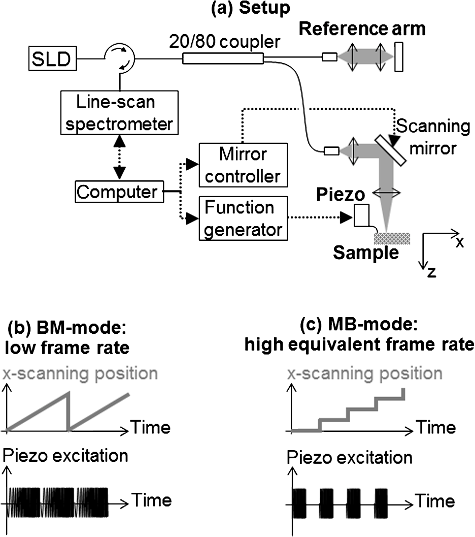

In the sample arm, a galvo-mirror scans the light beam laterally across the sample. The system can be operated in two scanning modes—either a conventional low-frame rate BM-mode [Fig. 1(a)] or a high-frame rate MB-mode [Fig. 1(b)]—as detailed in the following Secs. 2.2 and 2.3.

2.2.

Low-Frame Rate Shear Wave Imaging

2.2.1.

Conventional slow BM-mode

In the conventional BM-mode [Fig. 1(a)], A-lines are successively acquired at 256 adjacent locations by scanning the light beam across a 2.5-mm lateral imaging range, forming a two-dimensional image of the sample in the $(x, z)$ plane with a pixel size of $5 μ m \times 10 μ m$ ( $axial \times lateral$ ). Time-series of images are then acquired by repeating the B-scan 256 times while the sample is continuously and randomly vibrating without any synchronization with the acquisition. The displacements are retrieved from the phase difference between A-lines corresponding to a given location. This results in a movie of the displacements $u_{z} (x, z, t)$ at $190 frames / s$ with a total recording time of 1.4 s.

At such a low-frame rate, each frame corresponds to a different realization of a random displacement field. In other words, the acquisition is temporally incoherent. The lateral coherence is also low since different lateral locations are imaged sequentially. Nevertheless, the axial coherence of the displacement field is preserved since SD-OCT acquires depth profiles in a single shot, which allows to determine the wavelength of the shear wave using a cross-correlation approach.

2.2.2.

Shear wavelength tomography using a cross-correlation approach

The measured diffuse displacement field $φ (\vec{r_{0}}, t)$ can be expressed as a time-convolution product of the source function $s (\vec{r_{s}}, t)$ located at $\vec{r_{s}}$ and the impulse response $h$ of the propagation medium between the source location and a receiver located at $\vec{r_{0}}$

Eq. (2)

φ (\vec{r_{0}}, t) = s (\vec{r_{s}}, t) \overset{\otimes}{t} h (\vec{r_{0}}, \vec{r_{s}}, t) .

The time-reversed field

φ^{TR} (\vec{r}, t)

is simply computed by replacing the excitation function by the TR of the impulse response at a given location

\vec{r_{0}}

Eq. (3)

φ^{TR} (\vec{r}, t) = h (\vec{r_{0}}, \vec{r_{s}}, - t) \overset{\otimes}{t} h (\vec{r}, \vec{r_{s}}, t) .

Equation (2) can be generalized from a point-like impulse source to a time dependent with any spatial dimension source as follows:

Eq. (4)

φ^{TR} (\vec{r}, t) = φ (\vec{r_{0}}, - t) \overset{\otimes}{t} φ (\vec{r}, t) .

This expression is the generalized form of the TR field. It is known in seismology as coda wave interferometry³¹ and happens to be the spatiotemporal correlation from a signal processing point of view. In this approach, the Green’s function can be retrieved by a correlation between two measurement points of a broadband and diffuse wave field. This approach of TR is known as the monopole TR.³² It differs from the perfect TR in the way that it straightly expresses the impulse responses as a correlation. A perfect TR would be equivalent to a time derivative of the correlation,³³ either monopole or perfect. The TR approach developed in this section is not impacted by this latter time derivative.

The strain field $ξ_{z}$ , which is the spatial derivative of the wave field $φ$ in the source direction $z$ , also obeys the wave equation and can thus be expressed under the generalized TR form

Eq. (5)

{ξ_{Z}}^{TR} (\vec{r}, t) = ξ_{z} (\vec{r_{0}}, - t) \overset{\otimes}{t} ξ_{z} (\vec{r}, t) .

In our case, we use only a single spatial point, i.e., the source $\vec{r_{0}}$ at the focus time $t = 0$ . In an ideal isotropic diffuse field, the plane wave decomposition of a monochromatic plane wave $φ = e^{i k x}$ at this given frequency allows using the approximation of the strain as $ξ_{z} = i k φ$ , where $k$ is the wave number. It can be deduced that the two forms of the time-reversed fields [Eqs. (4) and (5)] are linked as follows:

Eq. (6)

ξ_{Z}^{TR} = - k^{2} φ^{TR} .

The local wavelength $λ$ can be estimated from the wave number $k$

Eq. (7)

λ (\vec{r_{0}}) ≅ 2 π \sqrt{- \frac{φ^{TR} (\vec{r_{0}}, t_{0})}{ξ_{Z}^{TR} (\vec{r_{0}}, t_{0})}} .

Shear wavelength tomography is then performed by determining the wavelength at each location

\vec{r_{0}}

of the imaging plane.

In practice, our algorithm proceeds as follows:

• The time-reversed displacement field (i.e., the energy of the displacement field) is determined by computing the spatiotemporal correlation of the displacement field and considering only the autocorrelation ( $\vec{r} = \vec{0}$ , $t = 0$ ).
• The strain field is deduced from the displacement field as $ξ_{Z} (\vec{r}, t) = \frac{φ (z - d z, t) - φ (z + d z, t)}{2 d z}$ . Then the time-reversed strain field is computed as the autocorrelation of the strain field.
• Afterward, the wavelength is deduced from the ratio between both time-reversed fields. No filter and no other processing are applied to the displacement field.

2.3.

High Frame Rate, Active Shear Wave Imaging

We performed active shear wave imaging experiments at a high frame rate as a control for comparison with the low-frame rate shear wave imaging experiments. The principle of ultrafast active shear wave imaging using SD-OCT has been detailed in previous studies.¹⁰ In brief, in the MB-mode [Fig. 1(a)], a series of 256 consecutive A-lines are acquired at $76,000 lines / s$ at one given location of the sample. Time-series are then repeated at 256 adjacent lateral locations covering a 2.5-mm lateral imaging range with a pixel size of $5 μ m \times 10 μ m$ ( $axial \times lateral$ ). The shear wave is actively induced and triggered at the beginning of each time-series. The axial displacements are retrieved from the phase difference between consecutive A-lines within a time-series. The concatenation of all time-series results in a stroboscopic movie $u_{z} (x, z, t)$ of the shear wave propagation consisting of $256 \times 256$ A-lines with a sampling rate of 76 kHz. The total acquisition time is 1 s.

The local propagation speed of the shear wave is then computed by performing time-correlations of displacements recorded at adjacent positions: $c_{shear} (x, z) = Δ x / Δ t$ where $Δ t$ is the time needed for the shear wave to travel a distance $Δ x$ ( $Δ x = 2 pixels = 20 μ m$ in our case). We used the normalized correlation coefficient as a metric of the speed estimation reliability: all speed values resulting from correlation with a normalized coefficient $\leq 0.9$ were ignored.

2.4.

Ex Vivo Experiments on a Tissue-Mimicking Phantom

A tissue-mimicking phantom was made of aqueous solutions containing agarose (Sigma Aldrich, St. Louis, Missouri) for stiffness control and ${TiO}_{2}$ microbeads for optical scattering. The sample was made of two halves of different stiffnesses: the stiffer half contained 2% agarose (w/v) while the softer half contained 1% agarose (v/w). Both parts contained 1% (w/v) of ${TiO}_{2}$ . Three experiments were performed:

1. A high frame rate shear wave imaging experiment with $76,000 lines / s$ imaging of high-frequency shear waves (500 to 6000 Hz). It served as a control to characterize the stiffness contrast between both parts of the phantom by computing shear wave speed maps. The shear wave was induced by a single piezoelectric actuator placed at the sample surface and excited by 2-ms chirp sweeping frequencies between 500 and 6000 Hz. The excitation was repeated synchronously with the acquisition as explained in Sec. 2.2. The resulting displacement field was processed using a pulse compression approach that provides broadband shear waves with high signal-to-noise ratio and high spatiotemporal resolution, as detailed in previous works.³⁴
2. A low-frame rate, diffuse shear wave imaging experiment with $190 frames / s$ imaging of high-frequency shear waves (500 to 6000 Hz). A random shear wave field was induced using two piezoelectric actuators placed on the sample surface and asynchronously excited with continuously repeated chirps (2-ms repetition period, frequency sweeping between 500 and 6000 Hz). The resulting wavelength map was compared with the expected values determined from the ultrafast experiment.
3. A slow, diffuse shear wave imaging experiment with $190 frames / s$ imaging of low-frequency shear waves (50 to 500 Hz) to reproduce the low frequency range expected for in vivo natural motions.

2.5.

In Vivo Experiments on the Eye of an Anesthetized Rat

A preliminary feasibility test was performed on the eye of an anesthetized rat (Long-Evans, Janvier Labs, Le-Genest-Saint-Isle, France). Animal manipulation was approved by the Quinze-Vingts National Ophthalmology Hospital and regional review board (CPP Ile-de-France V). The animal was anesthetized using injections of ketamine ( $40 mg / kg$ ) and Domitor ( $0.14 mg / kg$ ). In addition, the eye was locally anesthetized using oxybuprocaine chlorhydarate ( $1.6 mg / 0.4 mL$ ). The animal was positioned so that the eye faced the OCT light beam. Saline drops were periodically administered. Two experiments were performed:

1. A high frame rate, active experiment, where the shear wave was induced by a piezoelectric actuator gently placed on the sclera surface and tracked at $76,000 lines / s$ .
2. A low-frame rate, passive experiment, where natural vibrations of the eye (resulting from pulsatile motions) were imaged at $190 frames / s$ . Additionally, an ultrafast time-series was acquired (at $76,000 lines / s$ ) at one lateral location of the eye and its Fourier transform was computed to determine the spectral content of the natural vibrations.

3. Results

3.1.

Ex Vivo Experiments on a Tissue-Mimicking Phantom

3.1.1.

Recorded displacement field

Figure 2 shows the displacement field imaged in an agarose phantom at a sampling rate of either $76,000 lines / s$ using the MB-mode [Fig. 2(b)] or $190 frames / s$ using the BM-mode [Fig. 2(b)]. With the MB-mode, the piezoelectric actuator is placed at the left edge of the imaging plane and the displacement wavefront can be followed as it propagates from the left to the right. In the low-frame rate BM-mode, each frame shows a different realization of the random displacement field generated by two actuators placed on the sample surface from either side of the imaging area. It should be noted that the measured displacements are differential displacements occurring between two consecutive frames. Thus, the longer the time lapse between two consecutive frames, the higher the displacement’s magnitude. This is the reason why displacements appear with a higher magnitude in the BM-mode case, since the frame period is larger in the BM-mode than in the MB-mode. The displacement’s central frequency is 3500 Hz, as estimated by applying a Fourier transform to the displacements recorded in MB-mode (see Fig. 3).

Fig. 2

Snapshots of the displacement field recorded in an agarose phantom using either (a) the high frame rate MB-mode or (b) the low-frame rate BM-mode. The amplitude of the axial displacements (color scale) is overlaid on the morphologic image of the sample (gray scale). In both cases, the mechanical stimulation is a 2-ms chirp in the frequency range 500 to 6000 Hz, synchronized with the acquisition for the MB-mode and asynchronously repeated for the BM-mode.

Fig. 3

(a) Temporal profile of the axial displacements at one location of the phantom, detected at high imaging rate (76 kHz). (b) Corresponding spectrum. The central frequency is around 3500 Hz.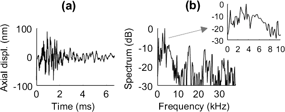

Because the imaging depth is limited to the surface of the phantom, the detected displacements likely correspond to surface waves, i.e., Rayleigh waves, which have a speed slightly lower than that of bulk shear waves: the Rayleigh wave speed is about 95% of the bulk shear wave speed.¹

3.1.2.

Characterization of the phantom using ultrafast shear wave imaging

The results of the ultrafast shear wave imaging experiment are shown in Fig. 4. The two parts of the sample can hardly be distinguished on the morphologic OCT image. However, the elastic wave speed map shows the stiffness contrast between both parts with a clear delineation at the interface. The Rayleigh wave speed is $7.5 \pm 2.9 m / s$ in the stiff part and $4.4 \pm 2.0 m / s$ in the soft part (median value ± standard deviation over regions of interest defined from the morphologic image). This is consistent with values reported in the literature.³⁵ There is, therefore, a 1.7 ratio between the speeds in both parts. Such speed values correspond to wavelengths values of 2.14 and 1.25 mm for, respectively, the stiff and the soft parts, at the central frequency of 3500 Hz (wavelength = speed/frequency). The lateral resolution of the stiffness map, defined as the width of the transition zone between both parts, is about $40 μ m$ .

Fig. 4

Results of an ultrafast shear wave imaging experiment in an agarose phantom with a broadband, high-frequency displacement field (500 to 6000 Hz). (a) Morphologic image of the phantom. The white arrow indicates the interface between the stiff (left) and the soft (right) parts of the phantom. (b) Shear wave speed map. (c) Lateral profile of the Rayleigh wave speed computed by averaging the speed over a $200 - μ m$ depth range.

3.1.3.

Shear wavelength tomography using low-frame rate shear wave imaging

Figure 5 shows the concept of shear wave time reversal using the cross-correlation approach. From the random displacement field shown in Fig. 2(b), we computed the time-reversed field at two different points of the sample, chosen, respectively, in the stiff ( $x 1 = 0.4 mm$ , $z 1 = 0.55 mm$ ) and the soft ( $x 2 = 1.26 mm$ , $z 2 = 0.55 mm$ ) parts of the phantom. Figures 5(a) and 5(b) show the spatial focusing obtained for each of the two locations at the time $t = 0$ of the cross correlation. The axial profile of these focal spots, shown in Fig. 5(c), highlight the fact that the focal spot size is bigger in the stiff part than in the soft part.

Fig. 5

Time-reversed displacement field computed using cross correlation for two different locations in the phantom. (a) and (b) Focal spots obtained at the two different locations. (c) Depth profile of the focal spot at the two locations (solid line = in the stiff part, dotted line = in the soft part). As expected, the size of the focal spot is larger in the stiff part than in the soft part.

The wavelength can be computed at each location of the imaging plane, yielding the wavelength map shown in Fig. 6. A significant contrast can be observed between the stiff and the soft parts of the phantom. An artifact due to the numerical spatial derivative of the wave field appears at the top of the shear wavelength map. The wavelength is $1.64 \pm 0.29 mm$ in the stiff part and $0.98 \pm 0.10 mm$ in the soft part (median value ± standard deviation over regions of interest defined from the morphologic image, excluding the artifact zone). There is, therefore, a 1.65 ratio between the wavelengths in both parts, which is consistent with the speed ratio measured in the ultrafast experiment. The measured wavelengths are of the same order of magnitude as the numbers obtained by converting the speed measurements into wavelengths values considering a central frequency of 3500 Hz for the displacement field. The variance of the wavelength measurements is lower than the variance of speed measurements, mostly because of a higher signal-to-noise ratio of the recorded displacements due to a higher displacement magnitude. The lateral resolution of the wavelength map, defined as the width of the transition zone between both parts, is about $100 μ m$ .

Fig. 6

Results of a low-frame rate shear wave imaging experiment in an agarose phantom with a broadband high-frequency shear wave (500 to 6000 Hz). (a) Morphologic image of the phantom. The white arrow indicates the interface between the stiff (left) and the soft (right) parts of the phantom. (b) Elastic wavelength map. (c) Lateral profile of the wavelength computed by averaging the wavelength over a $200 - μ m$ depth range.

We also assessed the feasibility of the cross-correlation approach with lower elastic wave frequencies, since in vivo passive elastography will rely on low frequency natural motions (generated by pulsatility). The results obtained with a diffuse displacement field in the frequency range 50 to 500 Hz are shown in Fig. 7. As expected, the wavelengths ( $2.09 \pm 0.6 mm$ in the stiff part and $1.34 \pm 0.14 mm$ in the soft part, median value ± standard deviation) are larger than that obtained with the high-frequency displacement field. The lateral resolution of the wavelength map ( $210 μ m$ ) is also lower than that obtained with the high-frequency elastic wave, but both parts can still be clearly identified as having significantly different stiffnesses, with a wavelength ratio of 1.56.

Fig. 7

Results of a low-frame rate shear wave imaging experiment in an agarose phantom with a broadband low-frequency elastic wave (50 to 500 Hz). (a) Morphologic image of the phantom. The white arrow indicates the interface between the stiff (left) and the soft (right) parts of the phantom. (b) Wavelength map. (c) Lateral profile of the wavelength computed by averaging the wavelength over a $200 - μ m$ depth range.

3.2.

In Vivo Experiments on the Eye of an Anesthetized Rat

We performed a preliminary in vivo experiment on the eye of an anesthetized rat. On the morphologic OCT image of the anterior segment of the eye [Fig. 9(a)], the following ocular tissues can be identified: cornea (co), sclera (sc), iris (ir), crystalline lens surface (le), and choroid (ch). Natural motions in the anterior segment of the rat eye were observed using the low-frame rate BM-mode (1.4 s recording time at $190 frames / s$ ), as shown in Fig. 8. These motions are induced by the animal heartbeat (pulsatile motions). The frequency range of the natural motions was estimated to 30 to 150 Hz in the different parts of the anterior segment.

Fig. 8

Snapshots of the natural motions recorded in the eye of an anesthetized rat using either the low-frame rate BM-mode. The amplitude of the axial displacements (color scale) is overlaid on the morphologic image of the eye (gray scale). The acquisition is completely passive: no active shear sources were used.

Fig. 9

Elastography performed on the eye of an anesthetized rat. (a) Different ocular tissues can be identified on the grayscale morphologic image: co, cornea; sc, sclera; le, lens; ir, iris; and ch, choroid. (b) Shear wave speed map resulting from a high frame rate, active shear wave imaging experiment (MB-mode). (c) Wavelength map resulting from a passive, low-frame rate shear wave imaging experiment (conventional BM-mode).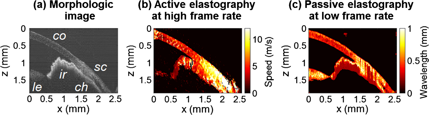

The cornea, the sclera, the iris, and the choroid are less than $500 - μ m$ thick, thus they are much thinner than the shear wavelength. In such a thin-layer configuration, shear waves are constrained by the layer boundaries and propagate in dispersive guided modes, which are sensitive to the layers’ thicknesses and the shear wave spectral content. Previous studies³⁶^,³⁷ have shown that Lamb-like modes are highly dispersive. A model refined for the cornea, called modified Rayleigh–Lamb equation, has recently been introduced to account for specific boundary conditions of the cornea,³⁵ and it also exhibits a highly dispersive behavior. The apparent speed (phase velocity) is lower than that in a bulk medium of equivalent stiffness (group velocity). In this case, studying the dispersion of the Rayleigh–Lamb-like wave propagation is required to quantitatively retrieve the tissue stiffness.

Nonetheless, a wavelength map [Fig. 9(b)] can be reconstructed from the displacement field induced by natural pulsatile motions. On this map, the sclera appears stiffer than the cornea with a clear delineation between both tissues at the limbus; and the choroid appears softer than the cornea and the sclera. The cornea seems to exhibit a stiffer upper layer, which could correspond to the epithelium. Figure 9(a) shows a speed map of the Lamb-like waves, which was obtained by performing an ultrafast active shear wave imaging experiment where a piezoelectric actuator was placed on the sclera (at the right edge of the imaging plane). As the ultrafast active and the passive experiments correspond to displacements with different spectral contents, the speed values obtained from the ultrafast active experiment cannot straightforwardly be compared with the wavelength values obtained from the passive experiments. As explained above, Rayleigh–Lamb-like modes tend to propagate with lower apparent speeds (and thus smaller wavelengths) than bulk shear waves. However, the relative stiffnesses of the cornea, the sclera, and the iris are consistent for both experiments.

A discrepancy between the ultrafast active and the low-frame rate passive experiments can be observed on the crystalline lens: the wavelength seems relatively high in the lens although it is expected to be much softer than other ocular tissues. This could be caused by particular boundary conditions related to the tissues’ geometry: the crystalline lens, unlike the other ocular structures, is not a thin-layered tissue. We think that the passive method measurements are related in the cornea to Lamb-like modes and in the crystalline lens to bulk shear waves. In other words, the wavelength contrast in this case is a consequence of a change of the wave regime rather than a change of stiffness. This effect is particularly strong for the passive approach because it relies on low-frequency waves, whereas the active SWE approach uses waves with high-frequency content and is, therefore, less sensitive to Lamb-like modes.

4. Discussion

Experiments performed on tissue-mimicking phantoms suggest that quantitative stiffness information can be retrieved by imaging a diffuse elastic wave field using low-frame rate SD-OCT. We obtained wavelength maps showing a clear contrast between the stiff and the soft parts of a heterogeneous phantom, with a wavelength ratio consistent with the speed ratio measured in ultrafast SWE. For a fair comparison, we generated the same spectral content (500 to 6000 Hz) in the shear wave field for both the noise-correlation experiment and the ultrafast SWE. However, as natural motions are expected to generate a much lower frequency range, we also performed the noise correlation with lower displacement frequencies (50 to 500 Hz). Consequently, we obtained higher wavelengths but a similar wavelength ratio between the stiff and the soft parts of the phantom.

In SWE, the spatial resolution depends on multiple parameters, including the shear wave frequency, the signal-to-noise ratio of the recorded displacements, and the spatiotemporal sampling of the shear wave propagation. In the ultrafast active SWE experiments presented above, we reached a lateral resolution of $40 μ m$ because both the lateral sampling ( $10 - μ m$ pixel size) and the temporal sampling ( $76,000 lines / s$ ) are high enough to detect speed changes within $40 μ m$ . In our noise-correlation approach, the spatial resolution is lower mainly because of the lower imaging rate ( $190 frames / s$ ). However, we still reach a resolution of hundreds of microns, which is much smaller than the millimeter-size shear wavelength.

The wavelength could be estimated directly by measuring the full-width-at-half-maximum of the focal spot of the time-reversed displacement field (see the two examples shown in Fig. 5). However, this method would require an imaging range covering the full size of the focal spot. On the contrary, with the algorithm described in this study, only three axial pixels are needed to compute the strain field.

As a first proof-of-concept for in vivo ophthalmic applications, we performed acquisitions on the eye of an anesthetized rat. Naturally induced elastic waves were observed in the cornea, the sclera, the iris, and the lens. Such natural motions do not perturb ultrafast active shear wave imaging, because they occur on longer time scales (hundreds of milliseconds) than the ultrafast recording time (a few milliseconds). An elastic wavelength map was reconstructed from the natural diffuse displacements and stiffness differences were observed between the cornea, the sclera, and the iris. However, extracting quantitative information requires accounting for the geometry of ocular tissues. Some parts of the eye are thin (hundreds of microns) compared with the shear wavelength (several millimeters) and act as wave guides that constrain the wave into Rayleigh–Lamb-like modes. In such a configuration, the propagation speed (and therefore the wavelength) depends not only on tissue stiffness, but also on tissue thickness and shear wave frequency.³⁷ The guidance effect being even stronger at low frequencies, it is essential to account for it for the case of passive elastography, which relies on natural motions (frequencies $< 200 Hz$ ). More detailed studies are planned to refine the reconstruction of quantitative elastic maps in such tissues from an analysis of the dispersion curve. Our preliminary results are, however, encouraging for the development of totally noninvasive stiffness mapping of the eye.

5. Conclusion

Stiffness information can be retrieved from imaging diffuse elastic waves using low-frame rate SD-OCT using a noise-correlation approach. The proof-of-concept was established on tissue-mimicking phantoms and a preliminary in vivo experiment was conducted on the eye of an anesthetized rat. The results open perspectives for in vivo passive elastography using conventional OCT systems. The envisioned biomedical applications include biomechanics studies of ocular tissues and skin layers. For that purpose, further studies will focus on refining the stiffness quantification in thin-layered tissue and to expand in vivo measurements.

Disclosures

I confirm that the authors report no financial interests or potential conflicts of interest.

Acknowledgments

This work was supported by the European Research Council SYNERGY Grant scheme (HELMHOLTZ, ERC Grant agreement No. 610110), Europe. The authors would like to thank Julie Degardin and Manuel Simonutti (Institut de la Vision, UPMC, Paris, France) for their help during the animal experimentation.

References

1.

D. Royer and E. Dieulesaint, Elastic Waves in Solids I: Free and Guided Propagation, Springer-Verlag, Berlin Heidelberg (2000). Google Scholar

2.

A. P. Sarvazyan et al., “Shear wave elasticity imaging: a new ultrasonic technology of medical diagnosis,” Ultrasound Med. Biol., 24 (9), 1419 –1435 (1998). http://dx.doi.org/10.1016/S0301-5629(98)00110-0 USMBA3 0301-5629 Google Scholar

3.

A. Manduca et al., “Magnetic resonance elastography: non-invasive mapping of tissue elasticity,” Med. Image Anal., 5 (4), 237 –254 (2001). http://dx.doi.org/10.1016/S1361-8415(00)00039-6 Google Scholar

4.

J. Bercoff, M. Tanter and M. Fink, “Supersonic shear imaging: a new technique for soft tissue elasticity mapping,” IEEE Trans. Ultrason. Ferroelectr. Freq. Control, 51 (4), 396 –409 (2004). http://dx.doi.org/10.1109/TUFFC.2004.1295425 ITUCER 0885-3010 Google Scholar

5.

K. Nightingale et al., “Acoustic radiation force impulse imaging: in vivo demonstration of clinical feasibility,” Ultrasound Med. Biol., 28 (2), 227 –235 (2002). http://dx.doi.org/10.1016/S0301-5629(01)00499-9 USMBA3 0301-5629 Google Scholar

6.

R. K. Wang, Z. Ma and S. J. Kirkpatrick, “Tissue Doppler optical coherence elastography for real time strain rate and strain mapping of soft tissue,” Appl. Phys. Lett., 89 (14), 144103 (2006). http://dx.doi.org/10.1063/1.2357854 APPLAB 0003-6951 Google Scholar

7.

R. K. Wang, S. Kirkpatrick and M. Hinds, “Phase-sensitive optical coherence elastography for mapping tissue microstrains in real time,” Appl. Phys. Lett., 90 (16), 164105 (2007). http://dx.doi.org/10.1063/1.2724920 APPLAB 0003-6951 Google Scholar

8.

S. Wang and K. V. Larin, “Shear wave imaging optical coherence tomography (SWI-OCT) for ocular tissue biomechanics,” Opt. Lett., 39 (1), 1 –4 (2014). http://dx.doi.org/10.1007/s11801-014-3177-9 OPLEDP 0146-9592 Google Scholar

9.

S. Song et al., “Strategies to improve phase-stability of ultrafast swept source optical coherence tomography for single shot imaging of transient mechanical waves at 16 kHz frame rate,” Appl. Phys. Lett., 108 191104 (2016). http://dx.doi.org/10.1063/1.4949469 Google Scholar

10.

S. Song et al., “Shear modulus imaging by direct visualization of propagating shear waves with phase-sensitive optical coherence tomography,” J. Biomed. Opt., 18 (12), 121509 (2013). http://dx.doi.org/10.1117/1.JBO.18.12.121509 JBOPFO 1083-3668 Google Scholar

11.

S. Wang et al., “Noncontact measurement of elasticity for the detection of soft-tissue tumors using phase-sensitive optical coherence tomography combined with a focused air-puff system,” Opt. Lett., 37 (24), 5184 –5186 (2012). http://dx.doi.org/10.1364/OL.37.005184 OPLEDP 0146-9592 Google Scholar

12.

J. Li et al., “Dynamic optical coherence tomography measurements of elastic wave propagation in tissue-mimicking phantoms and mouse cornea in vivo,” J. Biomed. Opt., 18 (12), 121503 (2013). http://dx.doi.org/10.1117/1.JBO.18.12.121503 JBOPFO 1083-3668 Google Scholar

13.

M. Singh et al., “Noncontact elastic wave imaging optical coherence elastography for evaluating changes in corneal elasticity due to crosslinking,” IEEE J. Sel. Top. Quantum Electron., 22 (3), 266 –276 (2016). http://dx.doi.org/10.1109/JSTQE.2015.2510293 IJSQEN 1077-260X Google Scholar

14.

M. Razani et al., “Feasibility of optical coherence elastography measurements of shear wave propagation in homogeneous tissue equivalent phantoms,” Biomed. Opt. Express, 3 (5), 972 –980 (2012). http://dx.doi.org/10.1364/BOE.3.000972 BOEICL 2156-7085 Google Scholar

15.

T.-M. Nguyen et al., “Visualizing ultrasonically induced shear wave propagation using phase-sensitive optical coherence tomography for dynamic elastography,” Opt. Lett., 39 (5), 838 –841 (2014). http://dx.doi.org/10.1364/OL.39.000838 OPLEDP 0146-9592 Google Scholar

16.

T.-M. Nguyen et al., “Shear wave elastography using amplitude-modulated acoustic radiation force and phase-sensitive optical coherence tomography,” J. Biomed. Opt., 20 (1), 016001 (2015). http://dx.doi.org/10.1117/1.JBO.20.1.016001 JBOPFO 1083-3668 Google Scholar

17.

C. Li et al., “Laser induced surface acoustic wave combined with phase sensitive optical coherence tomography for superficial tissue characterization: a solution for practical application,” Biomed. Opt. Express, 5 (5), 1403 (2014). http://dx.doi.org/10.1364/BOE.5.001403 BOEICL 2156-7085 Google Scholar

18.

C. Li et al., “Noncontact all-optical measurement of corneal elasticity,” Opt. Lett., 37 (10), 1625 (2012). http://dx.doi.org/10.1364/OL.37.001625 OPLEDP 0146-9592 Google Scholar

19.

Jr. T. L. Duvall et al., “Time–distance helioseismology,” Nature, 362 430 –432 (1993). http://dx.doi.org/10.1038/362430a0 Google Scholar

20.

P. M. Giles et al., “A subsurface flow of material from the Sun’s equator to its poles,” Nature, 390 52 –54 (1997). http://dx.doi.org/10.1038/36294 Google Scholar

21.

M. J. Buckingham, B. V. Berkhous and S. A. L. Glegg, “Passive imaging of targets with ambient noise,” Nat. London, 356 327 –329 (1992). http://dx.doi.org/10.1038/356327a0 Google Scholar

22.

P. Roux, B. D. Kuppermann and N. Group, “Extracting coherent wave fronts from acoustic ambient noise in the ocean,” J. Acoust. Soc. Am., 116 1995 –2003 (2004). http://dx.doi.org/10.1121/1.1797754 JASMAN 0001-4966 Google Scholar

23.

R. Weaver and O. Lobkis, “On the emergence of the Green’s function in the correlations of a diffuse field: pulse-echo using thermal phonons,” Ultrasonics, 40 435 –439 (2002). http://dx.doi.org/10.1016/S0041-624X(02)00156-7 ULTRA3 0041-624X Google Scholar

24.

H. Kanai et al., “Transcutaneous measurement and spectrum analysis of heart wall vibrations,” IEEE Trans. Ultrason. Ferroelectr. Freq. Control, 43 791 –810 (1996). http://dx.doi.org/10.1109/58.535480 ITUCER 0885-3010 Google Scholar

25.

E. E. Konofagou, J. D’Hooge and J. Ophir, “Myocardial elastography—a feasibility study in vivo,” Ultrasound Med. Biol., 28 475 –482 (2002). http://dx.doi.org/10.1016/S0301-5629(02)00488-X USMBA3 0301-5629 Google Scholar

26.

K. G. Sabra et al., “Passive in vivo elastography from skeletal muscle noise,” Appl. Phys. Lett., 90 (19), 194101 (2007). http://dx.doi.org/10.1063/1.2737358 APPLAB 0003-6951 Google Scholar

27.

T. Gallot et al., “Passive elastography: shear-wave tomography from physiological-noise correlation in soft tissues,” IEEE Trans. Ultrason. Ferroelectr. Freq. Control, 58 (6), 1122 –1126 (2011). http://dx.doi.org/10.1109/TUFFC.2011.1920 ITUCER 0885-3010 Google Scholar

28.

N. Benech et al., “Elasticity estimation by time-reversal of shear waves,” in Proc. IEEE Ultrasonics Symp., 2263 –2266 (2007). http://dx.doi.org/10.1109/ULTSYM.2007.569 Google Scholar

29.

S. Catheline et al., “Time reversal of elastic waves in soft solids,” Phys. Rev. Lett., 100 (6), 1 –4 (2008). http://dx.doi.org/10.1103/PhysRevLett.100.064301 PRLTAO 0031-9007 Google Scholar

30.

S. Catheline et al., “Tomography from diffuse waves: passive shear wave imaging using low frame rate scanners,” Appl. Phys. Lett., 103 (1), 014101 (2013). http://dx.doi.org/10.1063/1.4812515 APPLAB 0003-6951 Google Scholar

31.

N. M. Shapiro et al., “High-resolution surface-wave tomography from ambient seismic noise,” Science, 307 (5715), 1615 –1618 (2005). http://dx.doi.org/10.1126/science.1108339 SCIEAS 0036-8075 Google Scholar

32.

J. de Rosny and M. Fink, “Focusing properties of near-field time reversal,” Phys. Rev. A, 76 (6), 65801 (2007). http://dx.doi.org/10.1103/PhysRevA.76.065801 Google Scholar

33.

P. Roux et al., “Ambient noise cross correlation in free space: theoretical approach,” J. Acoust. Soc. Am., 117 (1), 79 –84 (2005). http://dx.doi.org/10.1121/1.1830673 JASMAN 0001-4966 Google Scholar

34.

T.-M. Nguyen et al., “Shear wave pulse compression for dynamic elastography using phase-sensitive optical coherence tomography,” J. Biomed. Opt., 19 (1), 016013 (2014). http://dx.doi.org/10.1117/1.JBO.19.1.016013 JBOPFO 1083-3668 Google Scholar

35.

Z. Han et al., “Quantitative assessment of corneal viscoelasticity using optical coherence elastography and a modified Rayleigh–Lamb equation,” J. Biomed. Opt., 20 (2), 020501 (2015). http://dx.doi.org/10.1117/1.JBO.20.2.020501 JBOPFO 1083-3668 Google Scholar

36.

M. Couade et al., “Quantitative assessment of arterial wall biomechanical properties using shear wave imaging,” Ultrasound Med. Biol., 36 (10), 1662 –1676 (2010). http://dx.doi.org/10.1016/j.ultrasmedbio.2010.07.004 USMBA3 0301-5629 Google Scholar

37.

T.-M. Nguyen et al., “Assessment of viscous and elastic properties of sub-wavelength layered soft tissues using shear wave spectroscopy: theoretical framework and in vitro experimental validation,” IEEE Trans. Ultrason. Ferroelectr. Freq. Control, 58 (11), 2305 –2315 (2011). http://dx.doi.org/10.1109/TUFFC.2011.2088 ITUCER 0885-3010 Google Scholar

Biographies for the authors are not available.

Citation Download Citation

Thu-Mai Nguyen, Ali Zorgani, Maxime Lescanne, Claude Boccara, Mathias Fink, and Stefan Catheline "Diffuse shear wave imaging: toward passive elastography using low-frame rate spectral-domain optical coherence tomography," Journal of Biomedical Optics 21(12), 126013 (21 December 2016). https://doi.org/10.1117/1.JBO.21.12.126013

Received: 24 August 2016; Accepted: 1 December 2016; Published: 21 December 2016

Access the abstract

JOURNAL ARTICLE
8 PAGES

DOWNLOAD PAPER SAVE TO MY LIBRARY

GET CITATION

CITATIONS

Cited by 36 scholarly publications.

Explore citations on Lens.org

RIGHTS & PERMISSIONS

Get copyright permission Get copyright permission on Copyright Marketplace

KEYWORDS

Tissues

Elastography

Optical coherence tomography

Eye

Wave propagation

Ultrafast imaging

In vivo imaging

1.

Introduction

2.

Materials and Methods

2.1.

Shear Wave Imaging Using Spectral-Domain Optical Coherence Tomography

Eq. (1)

Fig. 1

2.2.

Low-Frame Rate Shear Wave Imaging

2.2.1.

Conventional slow BM-mode

2.2.2.

Shear wavelength tomography using a cross-correlation approach

Eq. (2)

Eq. (3)

Eq. (4)

Eq. (5)

Eq. (6)

Eq. (7)

2.3.

High Frame Rate, Active Shear Wave Imaging

2.4.

Ex Vivo Experiments on a Tissue-Mimicking Phantom

2.5.

In Vivo Experiments on the Eye of an Anesthetized Rat

3.

Results

3.1.

Ex Vivo Experiments on a Tissue-Mimicking Phantom

3.1.1.

Recorded displacement field

Fig. 2

Fig. 3

3.1.2.

Characterization of the phantom using ultrafast shear wave imaging

Fig. 4

3.1.3.

Shear wavelength tomography using low-frame rate shear wave imaging

Fig. 5

Fig. 6

Fig. 7

3.2.

In Vivo Experiments on the Eye of an Anesthetized Rat

Fig. 8

Fig. 9

4.

Discussion

5.

Conclusion

Disclosures

Acknowledgments

References

Show All Keywords

Keywords/Phrases

Search In:

Publication Years