1.

Introduction

Human blood contains different type of cells; however, red blood cells (RBC) or erythrocyte are the most abundant cell type. RBC contains hemoglobin, which binds to either oxygen or carbon dioxide. This allows oxygen to be transported to tissues and organs and carbon dioxide to be taken away during microcirculation. The biconcave shape of the erythrocyte is extremely important in the functionality of RBCs. It allows the membrane to have a high surface area to volume (SAV) ratio facilitating large reversible elastic deformation of the RBC while squeezing through the tiny capillaries.^1–3 According to its importance, it has drawn considerable attentions into the pathology research in the clinical relevant blood diseases. Pathological disorders can modify RBCs and lead to significant alterations in its original shape.⁴ The consequences of modified RBC often are observed as clinical symptoms ranges from obstruction of capillaries and restriction of blood flow to tissues to necrosis and organ critical damages.^4–9 Also, counting cell types in the blood sample is another important task for investigating clinical status, which can be evaluated by well-known methods such as complete blood count or RBC distribution width, which are part of cytometry field. Because an automated cell counter samples and counts so many cells, the results are reliable in most of the cases.¹⁰ However, certain abnormal cells in the blood may not be identified correctly, requiring manual review and identification of any abnormal RBCs the instrument could not categorize. This information can be very helpful regarding identifying the cause of a patient’s anemia. Abnormal increase or decrease in RBC counts as revealed in a complete RBC count may indicate that you have an underlying medical condition that calls for further evaluation.

In the case of RBC, biconcaves are a substantial type in a healthy person, but there are other RBCs types with the different percentage varying between healthy and unhealthy persons. It has been shown that the percentages of different types of RBCs will be distinct according to the RBC diseases type.¹⁰ Accordingly, it is essential to measure the percentage of each RBC type in a blood sample consists of multiple RBCs for diagnosis and drug testing subjects. Typically, the diagnosing is performed by a human expert, and it shows some drawbacks, such as time-cost consuming and inaccuracy. Generally, experts visualize the sample in the images through a microscope based on their subjective knowledge from the viewpoint of intensity, morphology, texture, and so on based features. Usually, small-scale differences in the features are overlooked by human eyes especially for the border-line diagnostic scenario.

However, the situation has changed completely by the emergence of automatic classification algorithms. These techniques have been applied to problems in biology and have shown promising results for automatic recognition and classification of various micro-organisms.^11,12 Among the classification methods, the pattern recognition neural network (PRNN) has been suggested in nonlinear classification problems, such as RBC classification and counting.^13–15 The fundamental benefit of artificial neural network (ANN) is nothing, but it does not use any mathematical model since ANN learns from data sets and identifies patterns in a sequence of input and output data without any previous assumptions about their type and interrelations. Also, ANN eliminates the drawbacks of the conventional methods by extracting the wanted information using the input data.

In conventional RBC classification problems, the experts deal with two-dimensional (2-D) erythrocyte images obtained by conventional microscopes and cameras.^13,16–19 These methods generally have good performance but most of them have a significant number of features since they need to discriminate groups by utilizing 2-D features. However, in the case of RBC, which is transparent or semitransparent, we cannot take advantage of conventional intensity-based microscopes. Therefore, we believe that to obtain a satisfied level of accuracy, the classification and recognition should also take into account the three-dimensional (3-D) shape of RBCs. Among the techniques that can provide 3-D images of transparent or semitransparent cells, digital holographic microscopy (DHM) has shown promising results.^20–24 Also, the DHM technique has been utilized in the classification of RBC using 2-D and 3-D features since DHM can provide quantitative phase image.^25–27 In studying RBC, DHM enables the measurement of 3-D features, such as mean corpuscular volume, surface area, SAV ratio, functionality factor, sphericity index, and sphericity coefficients.^28,29 Chemical parameters of MCH and MCHSD can also be obtained due to DHM. Accordingly, we believe that any automated RBC classification that can distinguish different RBC types accurately should take into accounts the benefits of DHM imaging technique.

In this study, four main types of RBC shapes, biconcave (doughnut shape), flat discs, stomatocyte, and echinospherocyte are interested RBCs for the quantitative determination of the percentage of RBC types in multiple human RBCs. The reason for differentiating doughnut-shaped and flat-disc RBCs is that it can help in the applications of separating old cells versus young cells. It has been shown that during the stages of biconcave-echinocyte transformation in so-called storage lesion, biconcave cells become flat discs (loss of ATP results in a stiffer cytoskeleton that pulls the bilayer) after a few weeks of storage in blood bank.^29–34 Transfusion of these old samples might have critical consequences according to the previous studies.^35,36

At first, RBCs are visualized by off-axis DHM and the quantitative phase images are reconstructed by the numerical algorithm.^37,38 Then, single RBCs are extracted from images with multiple RBCs using the watershed algorithm.³⁹ At the next step, following 2-D features of projected surface area (PSA), perimeter, radius, elongation, and PSA to perimeter rate are extracted. In this paper, we have ignored extracting 2-D features related to the inner section of RBC, unlike the previous method proposed by Refs. 25, 26, since flat-disc and echinospherocyte RBCs do not have the inner section. Also, volume, surface area, SAV ratio, average RBC thickness, sphericity index, sphericity coefficient and functionality factors, and MCH and MCH surface density (chemical properties of RBC) are extracted from single RBCs. The latter feature-set is related to the morphological and biochemical properties of RBC 3-D profile. Along with the 3-D features, two new features related to the ring section of RBC are introduced. These features add significant information to the classification model and increase the discrimination power of the classifier. Then, each feature set is fed into PRNN, separately, and the classification results are compared using 10-fold cross validation (CV) technique. Since we are involved in a classification model with nonlinear decision boundary, we have decided to use PRNN strategy. In PRNN, the training algorithm is Bayesian regulation back-propagation, which updates the weights according to Levenberg–Marquardt optimization technique and the activation function for midlevel layers is hyperbolic tangent sigmoid.

Finally, to propose the best feature set, concerning both 2-D and 3-D features, sequential forward feature selection (SFFS) is utilized here. It has been shown that the best performance of a classification model can be achieved by selecting the most informative features and remove noisy ones that are either redundant or irrelevant.⁴⁰ Indeed, reducing the number of features can shorten training time, reduce the complexity of classifier, and simplify the model for interpretation goals. SFFS technique tries to select a subset of variables that best predict the data by sequentially selecting features until there is no improvement in the prediction.

In this paper, we have extracted 108 biconcave RBCs from a healthy sample stored for 1 day in the blood bank, 106 samples of stomatocyte shape from a sample with predominantly of stomato cells, 38 samples of flat-disc shape, and 71 samples of echinospherocyte shape for training and testing PRNN. Flat-disc and echinospherocyte cells are extracted from RBC samples stored in the blood bank for 40 days and 57 days, respectively. Performance comparison is evaluated by calculating misclassification rate of 10-fold CV technique. It is often claimed that leave-one-out-cross-validation (LOOCV) has higher variance than $k$-fold CV, and that it is because the training sets in LOOCV have more overlap. This makes the estimates from different folds more dependent than in the $k$-fold CV and, hence, increases the overall variance.⁴¹

Our experimental results demonstrate that the PRNN trained by 3-D features gives a good performance in classifying and counting RBCs in multiple human RBCs in an automated manner in comparisons with the 2-D features. In addition, we introduce the best set of features that combines 2-D and 3-D features to improve the RBCs classification accuracy. We believe that the final feature set evaluated with the presented neural network classification strategy can provide better discrimination results.

This paper is organized as follows. Section 2 explains the general scheme of the off-axis DHM to image RBCs and RBCs preparation. Section 3 explains 2-D and 3-D features extracted in this research and gives a short review about them. In Sec. 4, we will focus on designing the PRNN and counting different RBCs in multiple RBCs, automatically. The experimental results and discussions are provided in Sec. 5. Finally, the conclusion is presented in Sec. 6.

2.

Off-Axis Digital Holographic Microscopy and RBC Preparation

2.1.

Off-Axis Digital Holographic Microscopy

Figure 1 shows the off-axis DHM based on the Mach–Zehnder interferometer geometry.⁴² In this optical setup, light from a coherent source (HeNe laser diode source $\lambda =682\mathrm{nm}$) is split into reference and object beams by a beam splitter. The object beam is transmitted through the RBC sample and magnified by a $40\times /0.75$ NA microscope objective and interferes with the reference beam. The interference patterns between the diffracted object beam and the reference beam are recorded onto a CCD camera. The reconstruction of the RBC wavefront is obtained from the recorded hologram by using the numerical algorithm described in Refs. 37 and 38.

Fig. 1

Schematic representation of an off-axis DHM setup.

After reconstructing RBC phase images, single RBCs are extracted by the maker-controlled watershed segmentation algorithm.³⁹ Figure 2 shows a reconstructed phase image of a sample consisting of biconcave, flat-disc, and stomatocyte shape RBCs. This image shows that in a single sample it is possible to see RBC with different morphologies.

Fig. 2

Reconstructed image and three different RBCs inside. A is a flat disc RBC, B is a biconcave RBC, and C is a stomatocyte. White bar is $10\mu \mathrm{m}$.

3.

Feature Extraction

3.2.

Three-Dimensional Features

Since some 3-D features require thickness of the RBC, we first need to convert phase image into thickness image. Accordingly, the thickness value $h(i,j)$ for each pixel of $(i,j)$ with phase value $\varphi (i,j)$ in a phase image can be expressed as^28,29

Eq. (1)

$$h(i,j)=\frac{\varphi (i,j)\times \lambda }{2\pi (n_{\mathrm{rbc}}-n_m)},$$

where $\varphi (i,j)$ is the phase value in radians, and the refractive index of RBCs, $n_{\mathrm{rbc}}$, has been measured with a dual-wavelength DHM. Here, $n_{\mathrm{rbc}}$ is 1.396 with no significant difference among groups of RBCs. The index of refraction of the HEPA medium, $n_m$, is 1.3334. Surface area is another important property and has the main contribution in different 3-D features. Generally speaking, the surface area of the RBC is the surface area of the membrane mesh plus PSA. The method in this paper splits and divides RBC surfaces into smaller regular areas (triangles here) and adds these smaller areas to give the entire surface area. Understandably, the accuracy of such a calculation is dependent on the smaller area chosen.²⁹

3-D features listed in Table 1 are extracted in this paper. We only give a short description of the eight features related to the morphological properties of RBC, but interested readers can refer to Refs. 28 and 29 for the detail of each feature. Regarding the calculation of three features (F9-F11), we obtained many points over the ring section of RBC by applying two techniques. First, we estimate the ring section (blue triangles in Fig. 3) by calculating the radius of a circle having the area of the projection of RBC on $X\text{-}Y$ plane (the ring is around three-fourth of the RBC radius). Then, we update the position of each point on estimated ring (blue triangles) by finding the thickest point in a $3\times 3$ neighbor (red stars in Fig. 3). From now on we name the red stars as RPs. The single green point shows the center of RBC regarding the calculation of sphericity coefficient. In this study, we have decided to obtain 30 RP points. The reason is that the total number of points on the ring section for the stomatocyte RBCs is between 90 and 120 points according to our calculation. Also, since we are looking at a $3\times 3$ neighborhood around the blue triangles to find the point on the ring (red stars), there is high possibility of overlapping between red stars. For example, Fig. 4 shows the position of red stars and blue triangles when we increase the number of points. We can see that by increasing the number of red stars many of them overlap.

Table 1

3-D features descriptions.

	Feature name	Description
3-D-F1	AT	$\mathrm{AT}=\frac{\sum _{i=1}^k\sum _{j=1}^{l}h(i,j)}{k\times l}$ [$h(i,j)$ is the thickness at $(i,j)$’th pixel]
3-D-F2	Volume ($V$)	$V\cong p^2\sum _{i=1}^k\sum _{j=1}^{l}h(i,j)$
3-D-F3	TVS area	Surface area of the upper view of erythrocyte calculated by dividing surface into small triangles and then the summation of each triangle’s surface area
3-D-F4	TVS area volume ratio	$\mathrm{TVSV}=\frac{\mathrm{TVS}}{V}$
3-D-F5	Total surface area (SA)	$\mathrm{SA}=\mathrm{TVS}+\mathrm{PSA}$
3-D-F6	Surface area volume ratio (SAV)	$\mathrm{SAV}=\frac{\mathrm{SA}}{V}$
3-D-F7	Sphericity index (SI)	$\mathrm{SI}=\frac{4\pi V^{2/3}}{{(4\pi /3)}^{2/3}\mathrm{SA}}$
3-D-F8	Functionality factor (FF)	$f=\frac{\mathrm{SA}}{4\pi R^2}$
3-D-F9	Sphericity coefficient (SP)	$\mathrm{SP}=\frac{d_{\mathrm{c}}}{d_{\mathrm{r}}}$ ($d_{\mathrm{c}}$ and $d_{\mathrm{r}}$ are thickness values in RBC center and ring section, respectively)
3-D-F10	STD of thickness in ring section	This feature measures variation in the thickness of RPs in the ring of RBC
3-D-F11	Upper side of the ring/lower side of ring	This feature is calculated by dividing four maximum RPs by four minimums
3-D-F12	Mean hemoglobin (MCH)	$\mathrm{MCH}=\frac{10\overline{\varphi }(\mathrm{PSA})}{2\pi \alpha }$ ($\overline{\varphi }$ is the average phase value, $\lambda$ is the wavelength of the light source of the setup, and $\alpha =0.00196dl/g$ is a constant known as the specific refraction increment related to the protein concentration)
3-D-F13	MCH surface density (MCHSD)	$\mathrm{MCHSD}=\frac{\mathrm{MCH}}{\mathrm{PSA}}$

Fig. 3

3-D representation of four RBC categories and points on the ring section. (a) A typical biconcave sample, (b) a flat disc with center raised, (c) a stomatocyte RBC, and (d) a spherocyte RBC.

Fig. 4

3-D representation of RBC ring section with red stars and blue triangles on it. (a) Number of points is 60 and (b) number of points is 600.

We believe that earlier 3-D features can distinguish among different RBCs since they are related to the 3-D profile of RBC. The statistic $t$-test using two-sample Kolmogorov–Smirnov test revealed that some of these features are independent (data not shown). Table 2 shows average and STD values of each feature for each RBC type.

Table 2

3-D features (mean±STD).

	Biconcave	Flat-disc	Stomatocyte	Echinospherocyte
Average thickness ($\mu \mathrm{m}$)	$2.18\pm 0.3$	$2.27\pm 0.25$	$2.75\pm 0.36$	$4.47\pm 0.36$
Volume ($\mu {\mathrm{m}}^3$)	$93.23\pm 13$	$103.29\pm 14.72$	$95.85\pm 11.52$	$101.91\pm 16.4$
TVS area ($\mu {\mathrm{m}}^2$)	$103.85\pm 15$	$94.50\pm 9.62$	$106.04\pm 12.39$	$95.65\pm 10.6$
TVS area volume ratio ($\mu {\mathrm{m}}^{-1}$)	$1.12\pm 0.09$	$0.92\pm 0.05$	$1.11\pm 0.1$	$0.95\pm 0.06$
Total SA ($\mu {\mathrm{m}}^2$)	$148.32\pm 16.38$	$143.21\pm 12.48$	$147.32\pm 16.11$	$120.76\pm 11.79$
SA volume ratio ($\mu {\mathrm{m}}^{-1}$)	$1.61\pm 0.17$	$1.40\pm 0.13$	$1.55\pm 0.18$	$1.19\pm 0.09$
Sphericity index (SI)	$0.40\pm 0.18$	$0.74\pm 0.04$	$0.69\pm 0.06$	$0.87\pm 0.032$
Functionality factor (FF)	$0.86\pm 0.16$	$0.74\pm 0.07$	$0.93\pm 0.19$	$1.21\pm 0.14$
Sphericity coefficient (SP)	$0.67\pm 0.05$	$0.82\pm 0.06$	$0.5799\pm 0.21$	$1.16\pm 0.14$
STD of thickness in ring section	$0.0332\pm 0.021$	$0.054\pm 0.018$	$0.1321\pm 0.096$	$0.1254\pm 0.03$
Upper side of the ring/lower side of ring	$1.31\pm 0.11$	$1.25\pm 0.09$	$1.93\pm 0.44$	$1.44\pm 1.14$
MCH (pg)	$31.29\pm 4.55$	$34.68\pm 5.01$	$32.17\pm 3.94$	$34.29\pm 5.51$
MCHSD ($\mathrm{pg}/\mu {\mathrm{m}}^2$)	$0.68\pm 0.1$	$0.71\pm 0.08$	$0.85\pm 11$	$1.39\pm 0.11$

4.

Pattern Recognition Neural Network

ANNs are highly simplified mathematical models of biological neural networks having the ability to learn and provide meaningful solutions to the problems with high-level complexity and nonlinearity. The ANN approach is faster compared to its conventional techniques, robust in noisy environments, and can solve a wide range of problems. Due to the advantages, ANNs have been used in numerous applications.^13–15 A typical ANN is presented in Fig. 5. An important application of neural networks is pattern recognition that can be implemented by using a feed-forward neural network with a specific training function and specific function in the output layer. During training, the network is trained to associate outputs with input patterns. When the network is used, it identifies the input pattern and tries to output the associated output pattern.

Fig. 5

Feed-forward ANN configuration with five input nodes, two output nodes, and two hidden layers.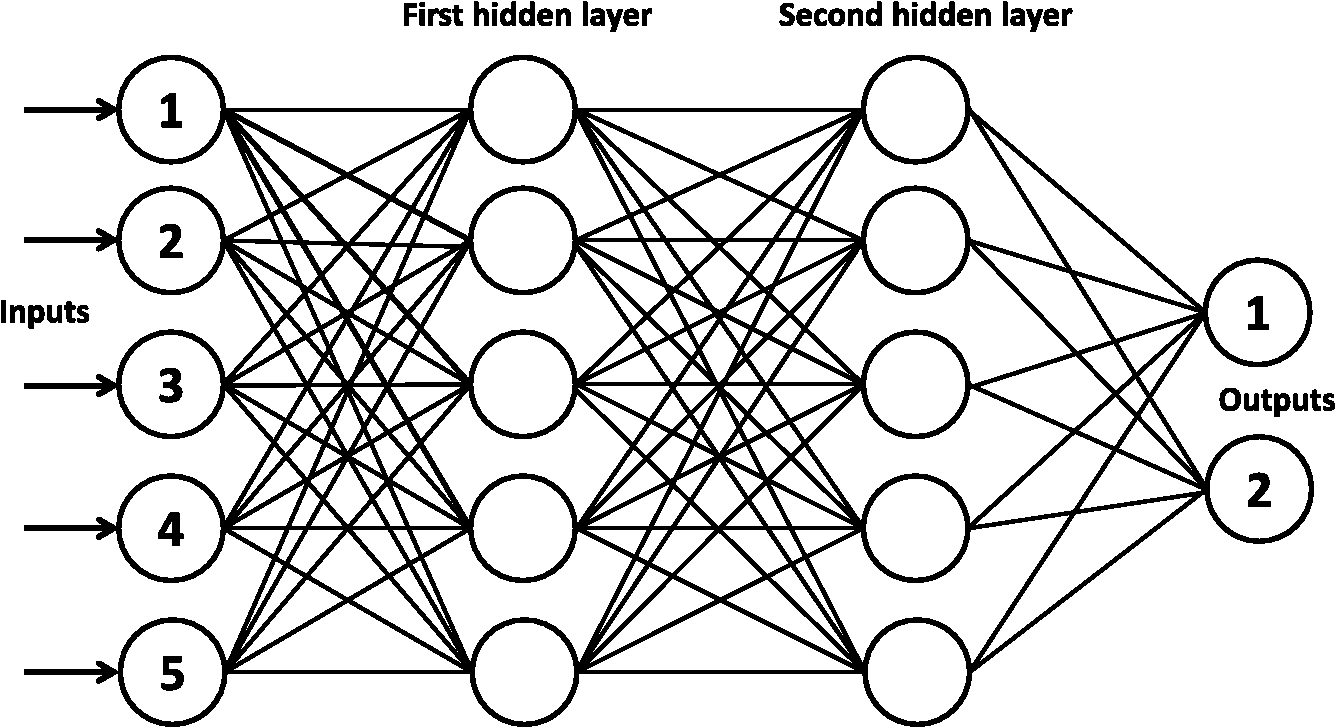

The information processing in the ANN strategy starts from the input layer to the hidden layer (from one hidden layer to another one if there are more than one) and from the last hidden layer to the output layer. A synaptic weight is assigned to each link to represent the relative connection strength of two nodes at both ends in predicting the input-output relationship. $y_j$ (the output) of any node $j$, is given as

For output layer in PRNN, the activation function is softmax transfer function (normalized exponential) that can be interpretable as posterior probabilities for a categorical target variable. It is highly desirable for those outputs to lie between zero and one and to sum to one. The purpose of the softmax activation function is to enforce these constraints on the outputs. Let the input to each output unit be $q_l$, $l=1,\dots ,k$, where $k$ is the number of classes. Then the softmax output $y_l$ is

5.

Experimental Results and Discussion

In this experiment, 108 RBCs are labeled as biconcaves, 106 RBCs labeled as stomatocytes, 38 RBCs are labeled as flat-disc, and 71 RBCs labeled as echinospherocytes. Four samples of each group are shown in Fig. 6. Simulations are all executed on a 64-bit Windows 7 computer with a 3.60-GHz Intel Core i7-4790 CPU, 8 GB RAM, and 8 cores. The performance of the classification model is assessed by utilizing 10-fold CV check. Put it simply, the data set is divided into 10 subsets, and the test is repeated 10 times. Each time, one of the 10 subsets is used as the test set and the other 9 subsets are put together to form a training set. Then, the average misclassification error across all 10 trials can show the overall misclassification error. PRNN consists of one input, output layer, and three hidden layers. Number of neurons in each hidden layer is 5, 10, and 5, respectively. Neuron numbers are obtained by trial-and-error technique. All the simulations codes are implemented in MATLAB^® 2014.

Fig. 6

Samples of each RBC group used in this research: (a) four samples of flat disks, (b) four samples of stomatocyte morphology, (c) four samples of biconcave RBC, and (d) four samples of spheroechinocyte RBC.

5.2.

Combining 2-D and 3-D Features and Select the Best Feature-Set

We believe that the best classification model should take into account not only 3-D features but also 2-D features. However, it is worth mentioning that not any feature can add significant information to the classification model. Therefore, we believe that the performance of any classification model can be enhanced by taking advantages of feature selection (FS) strategy. In FS, we seek to find the best set of the features that has the strongest ability (or strong) to distinguish each class. Generally speaking, FS preserves the original features intact; features deemed unimportant/irrelevant/redundant are simply eliminated from further consideration while selecting only those features that significantly contribute to the classification problem. Therefore, FS can reduce the number of features (variables) of the classification problem and make the model simpler (or less complex) and shorten training time.⁴⁰ We also implemented FS in this research by using SFFS technique. Generally speaking, in SFFS features are sequentially added to an empty candidate set until the addition of further features does not decrease the criterion. It has two components of an objective function, called the criterion, and a sequential search algorithm. In former, common criteria are misclassification rate for classification objects (similar in this paper) and mean squared error for regression models. A sequential forward search algorithm adds features from a candidate subset while evaluating the criterion. Since an exhaustive comparison of the criterion value at all $2^n$ subsets of an $n$-feature data set is typically infeasible (sometimes feasible but time-consuming), sequential searches grow the candidate set. It turns out that the following features of average RBC thickness (3-D-F1), top view surface (TVS) area volume ratio (3-D-F4), sphericity coefficient (3-D-F9), the upper side of the ring divided by lower side of the ring (3-D-F11), and perimeter (2-D-F2) can better classify multiple RBCs in this research. Our experimental results also show that adding more features does not add significant discrimination ability to the final classification model. As it has been mentioned earlier, SFFS is responsible for adding or removing features from the final feature set. One component of SFFS is the objective function, which here is the misclassification rate. SFFS starts from an empty set and add features one by one to the set and evaluates the misclassification rate. If there is a significant change in the objective function (misclassification rate) then the feature can be added to the final feature set (see Table 6).

Table 6

Misclassification rate after adding each feature to the feature set.

Features added to the set	Criterion value (misclassification rate)
Average RBC thickness (3-D-F1)	0.252396
RBC perimeter (2-D-F2)	0.134185
TVS area-volume ratio (3-D-F4)	0.0670927
Sphericity coefficient (3-D-F9)	0.0607029
The upper side of the ring divided by lower side of the ring (3-D-F11)	0.0511182
Adding next feature to the feature set (sixth feature)	0.479233
Adding next feature to the feature set (seventh feature)	0.479233
Adding next feature to the feature set (eighth feature)	0.479233

According to Table 6 after adding the 7th and 8th features, the misclassification rate never changes. It means that they have no contribution to the final feature set. Adding the 6th feature decreases the misclassification rate marginally but we still did not consider it as part of the feature set since we wanted to keep the final feature set as small as possible (only five features).

Figure 7 shows the data distribution RBCs for each selected feature. We can see that the distribution of average RBC thickness of echinospherocyte RBCs has almost no overlap with other distributions [Fig. 7(a)]. Table 7 shows misclassification rate of the final feature-set and PRNN approach.

Fig. 7

Data distribution of the best feature set. (a) Average thickness value. (b) Sphericity coefficient. (c) Upper side of the ring/lower side of the ring. (d) Top view surface area volume ratio. (e) Perimeter.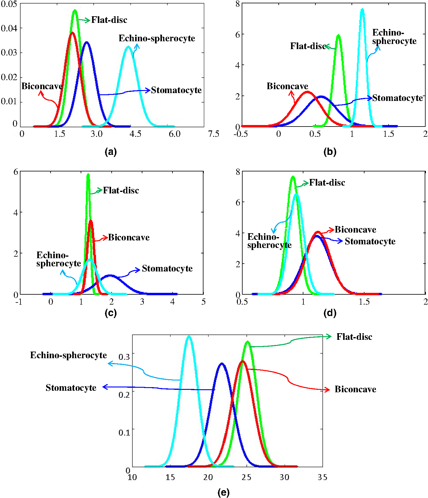

Table 7

Misclassification results for the best feature set obtained by sequential features selection technique.

	Flat-disc	Stomatocyte	Biconcave	Echinospherocyte
Best feature set	0%	0.9%	3.1%	0%

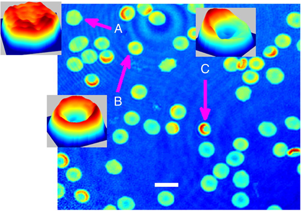
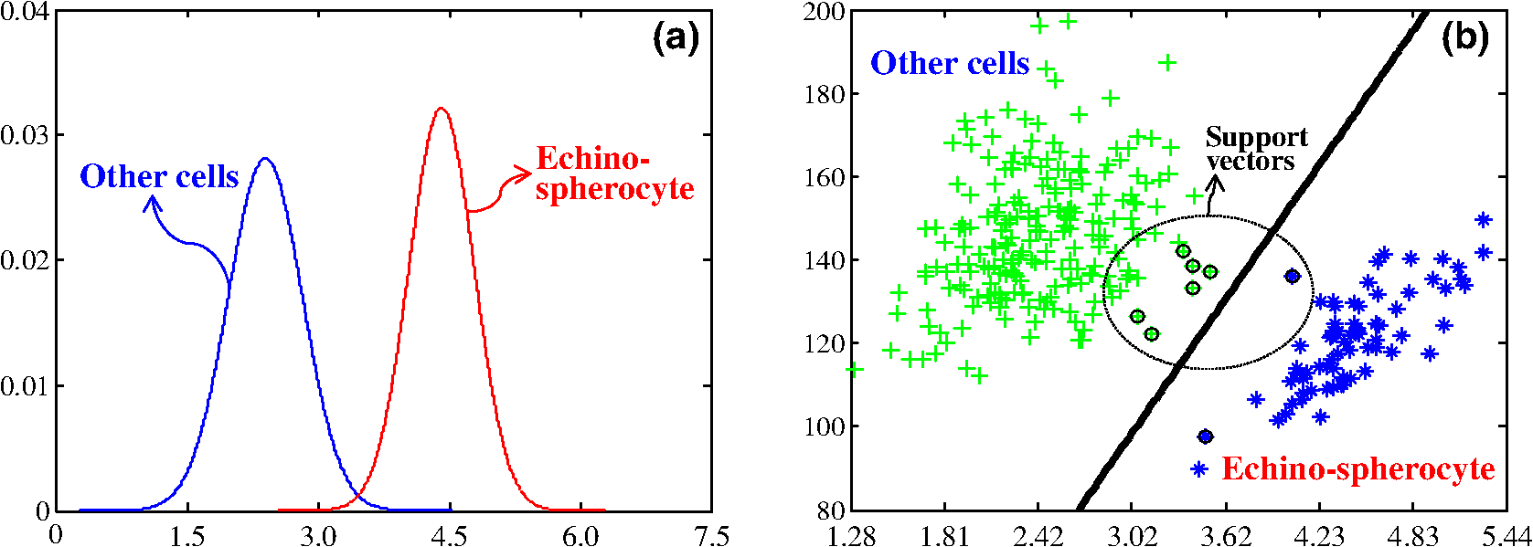
The confusion matrix of the test set shows that PRNN sometimes confuses stomatocytes and echinospherocytes because there are cases in which RBC has a morphology similar to both stomatocyte and echinospherocytes (see Fig. 8). According to Fig. 8, we can see that RBC is similar to both stomatocyte and echinospherocytes morphology and posterior probability for belonging to stomatocyte and echinospherocyte categories are 0.33 and 0.66, respectively. Even for a human examiner, it can be difficult to put it in the correct category.

Fig. 8

An RBC sample that confuses neural network, resembles both stomato and spherocyte. (a) 3-D representation and (b) representation on $X\text{-}Y$ plane.

In another experiment, we tried to count different types of RBCs in five quantitative phase images with multiple RBCs. Images are inspected visually by the human inspector and then results are presented. In Fig. 9(a) stomatocyte RBCs are dominant (flat discs 0/80, stomatocytes 58/80, biconcave 8/80, and echinospherocyte 14/80) and in other images biconcave RBCs [Fig. 9(b) has following flat discs 2/27, stomatocytes 5/27, biconcave 20/27, and echinospherocyte 0/27] and echinospherocytes are dominant [Fig. 9(c) shows RBC types of flat-disc 0/49, stomatocytes 5/49, biconcaves 6/49, and echinospherocytes 38/49, and Fig. 9(d) shows RBC types of flat-disc 0/63, stomatocytes 3/63, biconcaves 1/63, and echinospherocytes 59/63]. Figure 9(e) shows an image with 40 days storage time with many flat-disc RBCs (flat-disc: 16/36, stomatocytes: 7/36, biconcaves: 5/36, and echinospherocytes: 8/36). The numbers in parenthesis show the number of each morphology obtained by the human inspector. At first, each image is segmented into many RBCs since feature extraction should be applied at the single cell level. Then, the percentage of the different types of RBCs in the RBC phase images is calculated (see Fig. 9). As expected, the classifier showed that at the first sample stomatocyte RBCs are dominant. In contrast, in the second and fifth figures biconcave and flat-disc RBCs are the major types. Third and fourth figures illustrate that echinospherocytes are dominant RBCs. Although there is a small error in counting nondominant RBCs, the main and important thing is counting and reporting the dominant type for further investigation.

Fig. 9

Five RBC samples and counting results. (a) Flat-disc: 0%, stomatocytes: 76.2% (61/80), biconcave: 11.25% (9/80), and echinospherocyte: 10% (8/80). (b) Flat-disc: 7.40% (2/27), stomatocytes: 18.51% (5/27), biconcave: 74.07% (20/27), and echinospherocyte: 0%. (c) Flat-disc: 0%, stomatocytes: 12.24% (6/49), biconcave: 10.2% (5/49), and echinospherocyte: 77.55% (38/49). (d) Flat-disc: 0%, stomatocytes: 7.94% (5/63), biconcave: 1.59% (1/63), and echinospherocyte: 90.4% (57/63). (e) Flat-disc: 47.22% (17/36), stomatocytes: 25% (9/36), biconcave: 19.5.2% (7/36), and echinospherocyte: 8.3% (3/36).

According to the results, the proposed feature set and classifier can automatically count and categorize different types of RBCs in human RBCs by taking advantages of 2-D and 3-D profiles of RBC. The classifier is helpful to assess RBC-related abnormality since the ratio of the different types of RBCs is associated with certain types of diseases. There are some disadvantages in using NN technology regarding the classification such as there is no formula for the number of nodes and hidden layers. Generally, these numbers in the network are problem dependent and are decided by the trial-and-error method.

We believe that DHM, by providing the quantitative phase images, allows for doing different analysis especially classification goals. For example, someone can easily classify echino-echino-spherocyte from the rest of cells easily by using a conventional binary support vector machine (SVM) classifier and one or two features. Figure 10(a), e.g., shows the density of average cell thickness of echinospherocytes against other RBCs. Any binary classifier can be used to separate these two groups. Figure 10(b) shows the scattering of two groups based on average thickness (AT) value and surface area, and an SVM classifier with its boundary region.

Fig. 10

(a) AT value distribution for echinospherocytes and other RBCs and (b) an SVM classifier to separate echinospherocytes and other cells using AT and total surface area.

6.

Conclusions

Automatic classification of different types of RBCs in human RBC is a challenging and important problem for pathological diagnosis. In particular, as far as RBCs are concerned, classification based on their 3-D profile is highly relevant. Another issue is that since demands on laboratories are ever increasing and funding and staffing levels are generally below the desired level, the implementation of a system that shortens staff time, cost-effective, and noninvasive is greatly desired. In this paper, we have presented and assessed the use of PRNN applied to the 2-D and 3-D features of RBCs obtained through DHM in order to categorize and count biconcave, stomatocyte, flat-disc, and echinostomatocyte RBCs in an RBC sample with multiple types. Six 2-D features and 13 3-D features have been extracted and classification results are compared right after. Our experimental results show that the 3-D features have more useful information in RBC classification. In addition, FS shows that average RBC thickness, TVS area volume ratio, sphericity coefficient, the upper side of the ring divided by lower side of the ring, and RBC perimeter can better classify RBCs into the desired categories. The experimental results and the performance imply that the final feature set can help in classifying and counting RBCs, which is substantially important in analyzing RBC abnormality and shape-related diseases.