Automated choroid segmentation in three-dimensional 1-μm wide-view OCT images with gradient and regional costs

Fei Shi; Bei Tian; Weifang Zhu; Dehui Xiang; Lei Zhou; Haobo Xu; Xinjian Chen

doi:10.1117/1.JBO.21.12.126017

22 December 2016 Automated choroid segmentation in three-dimensional 1-μm wide-view OCT images with gradient and regional costs

Fei Shi, Bei Tian, Weifang Zhu, Dehui Xiang, Lei Zhou, Haobo Xu, Xinjian Chen

Author Affiliations +

Journal of Biomedical Optics, Vol. 21, Issue 12, 126017 (December 2016). https://doi.org/10.1117/1.JBO.21.12.126017

Abstract

Choroid thickness and volume estimated from optical coherence tomography (OCT) images have emerged as important metrics in disease management. This paper presents an automated three-dimensional (3-D) method for segmenting the choroid from 1-μm wide-view swept source OCT image volumes, including the Bruch’s membrane (BM) and the choroidal–scleral interface (CSI) segmentation. Two auxiliary boundaries are first detected by modified Canny operators and then the optical nerve head is detected and removed. The BM and the initial CSI segmentation are achieved by 3-D multiresolution graph search with gradient-based cost. The CSI is further refined by adding a regional cost, calculated from the wavelet-based gradual intensity distance. The segmentation accuracy is quantitatively evaluated on 32 normal eyes by comparing with manual segmentation and by reproducibility test. The mean choroid thickness difference from the manual segmentation is 19.16±4.32 μm, the mean Dice similarity coefficient is 93.17±1.30%, and the correlation coefficients between fovea-centered volumes obtained on repeated scans are larger than 0.97.

1. Introduction

The human choroid is a complex vascular structure lying between the retina and the sclera. It provides oxygen and nourishment to the outer layers of the retina, including the photoreceptor cells crucial to visual function.¹ The choroid morphology is relevant to many factors, such as age, gender, axial length, and intraocular pressure in healthy eyes.²^,³ Changes in the choroid, often manifested as changes in thickness and volume, are also associated with various ocular disorders, such as glaucoma,⁴ high myopia,⁵ age-related macular degeneration,⁶ central serous chorioretinopathy,⁷ and Vogt–Koyanagi–Harada disease.⁸ Accurate quantification of the choroid thickness or volume is of great interest in pathophysiology studies of these diseases.

Recent development of optical coherence tomography (OCT) has made several techniques available for high-speed and in vivo cross-sectional imaging of the choroid structure. The enhanced depth imaging OCT (EDI-OCT) obtains high signal strength by placing the “zero delay line” near the outer retina and choroid and enhances the signal-to-noise ratio (SNR) by averaging high number of B-scans.⁹ High-definition OCT (HD-OCT) can also be achieved by averaging selected high-quality B-scans in conventional 840-nm spectral domain OCT.³ However, in both EDI-OCT and HD-OCT, the requirement of averaging limits the number of B-scans finally obtained. Therefore, the choroid volume cannot be accurately calculated. Another recently introduced technique is the swept-source OCT (SS-OCT) with a central wavelength near $1 μ m$ .¹⁰ The longer wavelength allows better penetration through the deeper layers. As a result, a three-dimensional (3-D) volume showing both the retina and the entire choroid can be obtained. Along with the improved scanning speed, the wide-view scanning can include both the optical nerve head (ONH) and the macula. Two B-scans obtained by 1050-nm SS-OCT are shown in Fig. 1. Compared to EDI-OCT and HD-OCT, the 3-D image has higher level of speckle noise, which poses more difficulty for accurate segmentation.

Fig. 1

B-scan of 1050-nm wide-view SS-OCT image: (a) an original B-scan from SS-OCT image volume and (b) the same B-scan with several structure manually labeled.

The goal of automatic choroid segmentation is to delineate the Bruch’s membrane (BM) as the upper boundary and the choroidal–scleral interface (CSI) as the lower boundary, as shown in Fig. 1. The BM is the lower boundary of the retinal pigment epithelium (RPE) with high reflectivity, which is often detected by finding the maxima in intensity or gradient. On the contrary, the CSI can only be observed as the boundary between the textured region of choroid and the uniform region of sclera. It is often weak, broken, and open to subjective interpretation. Hence, the segmentation of CSI is far more challenging.

Some studies on automatic choroid segmentation have been carried out based on the aforementioned choroid imaging techniques. For EDI-OCT images, Tian et al.¹¹ detected “valley pixels” as local minima of A-scans and found CSI as the shortest path using Dijkstra’s algorithm. Alonso-Caneiro et al.¹² calculated a dual brightness probability gradient following image enhancement, which was used to form the weights to search for the CSI. Vupparaboina et al.¹³ measured the structural dissimilarity between choroid and sclera by structural similarity index and achieved final delineation by thresholding and tensor voting. Danesh et al.¹⁴ employed the wavelet-based features to construct a Gaussian mixture model, which was then used in a graph cut method for segmentation of CSI. Chen et al.¹⁵ used a graph-based method for delineating CSI in which both the searching space and the cost were obtained based on vasculature characteristics. Chen et al.¹⁶ also proposed a method based on gradual intensity distance for choroid segmentation in HD-OCT images. These are all two-dimensional (2-D) methods applied on images with high SNR. No 3-D context is used in segmentation, and most of them do not work well for images with low SNR. Studies on 3-D OCT volumes are limited. Hu et al.¹⁷ applied a 3-D multistage multisurface graph search method for choroid segmentation of highly anisotropic and high-SNR OCT volumes obtained by B-scan averaging. Kajic et al.¹⁸ used a statistical model based on texture and shape to automatically detect the choroid boundaries in the 1060-nm OCT B-scans of both healthy and pathological eyes. However, the method required extensive training. Zhang et al.¹⁹ proposed a 3-D method by which the CSI was identified by fitting a thin plate spline to the lower boundary of segmented choroidal vessels. It was later validated on both EDI-OCT and SS-OCT volumes by Philip et al.²⁰ Zhang et al.²¹ also proposed a method based on combined graph-cut-graph-search method and yielded accurate segmentation results for choroid surface segmentation in SS-OCT volumes. But the 3-D graph construction was complicated and the method was computationally expensive. In addition, manufacturer-provided segmentation software are also available for choroid thickness analysis,²² but failures are often observed²³ and manual correction is needed.

In this paper, we propose a 3-D automatic choroid segmentation method for 1050-nm wide-view SS-OCT volumes. The 3-D context is taken into consideration in the segmentation. A choroid thickness map and the choroid volume can be calculated from the segmentation results. The choroid both below the fovea and near the ONH can be segmented, which gives more information than methods based on the conventional macula-centered OCT images. The method works with images with relatively high speckle noise level.

In preprocessing, we propose to use linear mapping and a cross bilateral filtering to enhance the image quality. In the segmentation, modified Canny operators are used to detect two auxiliary boundaries. Based on the second boundary, the ONH is detected and the corresponding A-scans are excluded in the following procedures. The 3-D multiresolution graph search method is applied to achieve segmentation of the BM and CSI. For CSI, we propose the wavelet-based gradual intensity distance cost. Combined with the conventional gradient-based cost, accurate segmentation is obtained, even with weak and broken boundaries. The segmentation accuracy is quantitatively evaluated by comparing with manual segmentation and by reproducibility test.

2. Materials and Methods

3-D OCT volumes were acquired using a Topcon Swept Source OCT scanner at 1050 nm (DRI OCT-1 Atlantis, Topcon, Tokyo), with $20 - μ m$ lateral resolution and $8 - μ m$ axial resolution. The image size is $512 (width of B-scans) \times 256 (number of B-scans) \times 992 (depth of B-scans)$ , which corresponds to a $12 \times 9 \times 2.6 {mm}^{3}$ volume. In this paper, we define $x$ as the width index, $y$ as the B-scan index, and $z$ as the depth index, and a B-scan image is in the $x - z$ plane. Three data groups were constructed. Both eyes from 16 normal subjects were scanned twice within 10-min intervals, and formed groups A and B for reproducibility evaluation. Another 10 eyes from 5 normal subjects were scanned once, and formed group C for parameter optimization. For each image volume in groups A and C, 10 B-scans with even spacing (25 B-scans apart) were manually segmented by two experts. The average position of the manual delineation was used as ground truth (GT) for BM and CSI. The study was approved by the Institutional Review Board of Soochow University, and informed consent was obtained from all subjects.

2.1.

Image Enhancement

To work with an image with relatively high speckle noise level, two procedures are used to enhance the image quality.

1. Contrast enhancement by linear mapping. The intensities below a threshold are mapped to 0, and the maximum intensity is mapped to 1. The threshold is set as the mean of the background region, calculated from the image volume with 200 voxels in height in the lower part of the image. This mapping suppresses noise with low intensities and enhances the contrast between the bright layers with the dark background and the choroid vessel regions.
2. Speckle noise reduction by cross bilateral filtering. Bilateral filtering, with its edge-preserving ability, is often used for speckle noise reduction in OCT images.²⁴^,²⁵ It is essentially a local weighted averaging. The weights are the product of two Gaussian kernels, related to distance and intensity, respectively. The bilateral filtering is computed as follows:²⁶
Eq. (1)
$g (i, j) = \frac{\sum_{k, l} f (k, l) ω (i, j, k, l)}{\sum_{k, l} ω (i, j, k, l)},$
Eq. (2)
$ω (i, j, k, l) = d (i, j, k, l) r (i, j, k, l),$
Eq. (3)
$d (i, j, k, l) = \exp [- \frac{{(i - k)}^{2} + {(j - l)}^{2}}{2 σ_{d}^{2}}],$
Eq. (4)
$r (i, j, k, l) = \exp [- \frac{{‖ f (i, j) - f (k, l) ‖}^{2}}{2 σ_{r}^{2}}],$
where $f$ is the original image, $g$ is the filtered image, $(i, j)$ and $(k, l)$ are the pixel coordinates, and $σ_{d}^{2}$ and $σ_{r}^{2}$ are the variances of Gaussian kernels controlling the smoothness. However, the conventional bilateral filtering is better at removing Gaussian-like noise than the impulse-like noise, i.e., pixel with particularly higher or lower intensities than its neighbors. In the latter case, $r (i, j, k, l)$ will be small, and the total weight $ω (i, j, k, l)$ will also be small, thus resulting in insufficient averaging. Therefore, we propose to use a cross bilateral filter that incorporates the ability of the median filter in removing impulse noise. Equation (4) is then modified to Eq. (5), where $f_{M}$ is the result of median filtering of $f$ .
Eq. (5)
$r (i, j, k, l) = \exp [- \frac{{‖ f_{M} (i, j) - f_{M} (k, l) ‖}^{2}}{2 σ_{r}^{2}}] .$
The median-filter-guided cross bilateral filtering combines the advantage of both filters, which both reduces the speckle noise and preserves the edges. Here we apply a fast approximation technique,²⁷ where the filter is formulated in a higher dimensional space as convolution followed by simple nonlinear operations.

Part of a B-scan before and after the two-step image enhancement is shown in Fig. 2.

Fig. 2

Part of a B-scan (a) before and (b) after image enhancement and (c) image denoising.

2.2.

Optical Nerve Head Detection

Inside the ONH, most of the retinal layers, including RPE and CSI, are discontinuous. Therefore we detect the region first and remove it from the volume of interest (VOI). This also involves two steps:

1. Auxiliary boundary detection. We define two auxiliary surfaces. Surface 1 is the inner limiting membrane and also the upper boundary of nerve fiber layer. Surface 2 is the upper boundary of photoreceptor–RPE complex. These are two boundaries with the most notable dark-to-bright transitions. We detect them in each B-scan using two modified Canny edge detectors, according to their different morphologies.
The Canny edge detector calculates the gradient $G = (G_{x}, G_{z})$ in a smoothed image, and uses both the magnitude and direction of $G$ to determine the correct edge points.²⁸ Here, we use two types of modified gradient magnitude for detecting the two boundaries. As both of them are dark-to-bright edges, voxels with negative vertical component $G_{z}$ are considered. For surface 1, as the boundary drops suddenly in the ONH and $G_{z}$ will be close to zero, the horizontal component $G_{x}$ is also needed. Therefore, we use the following calculation for surfaces 1 and 2, respectively, and obtain two edge maps $E_{1}$ and $E_{2}$ , as shown in Fig. 3.
Eq. (6)
${| G |}_{1} = | G_{x} | + | \min (0, G_{z}) |,$
Eq. (7)
${| G |}_{2} = | \min (0, G_{z}) | .$
The modified Canny detectors constrain the type of edges detected and effectively remove interfering edge points. Then, the first edge point in each A-scan of $E_{1}$ is detected to form surface 1, for which median filtering is used to remove outliers. The first edge point below surface 1 in each A-scan of $E_{2}$ is detected to form surface 2, which will be further processed in the next step. The two edge maps are shown in Figs. 3(a) and 3(b), overlaid on the original B-scan.
2. ONH detection. The absence of edge below surface 1 in $E_{2}$ indicates the ONH region. Therefore, considering all the A-scans in the image volume, we can get a 2-D binary map, where white represents the A-scans inside the ONH, as shown in Fig. 4. The holes inside are caused by detection of the horizontal boundary of lamina cribrosa. Some small regions also appear caused by minor discontinuities in the detected surface 2. Postprocessing, including small region removing and hole filling, is applied to get the ONH, and the convex hull is calculated to smooth the boundary.

Fig. 3

Detection of two boundaries using modified Canny edge detectors: (a) edge map $E_{1}$ to detect surface 1, (b) edge map $E_{2}$ to detect surface 2. Note that vertical edges do not present in $E_{2}$ . (c) Detection results of surfaced 1 and 2, shown as red and green curves. Vertical yellow lines indicate the detected ONH region.

Fig. 4

ONH detection: (a) 2-D map obtained from detecting absence of surface 2, (b) after removing small regions and hole filling, and (c) final result obtained using convex hull.

Finally, all the discontinuities in surface 2, including ONH, are removed by linear interpolation. This surface, as shown in Fig. 3(c), is used to constrain the BM segmentation in the next section.

2.3.

BM and CSI Segmentation

The BM is a boundary with bright-to-dark transition at the bottom of the retina. Although the CSI is not a clear boundary, in most places it appears as the bottom of large choroidal vessels. Therefore, we get the initial segmentation by assuming it as a dark-to-bright boundary. Since the BM and CSI are less notable transitions than surfaces 1 and 2, a 3-D multiresolution graph search method is used for the segmentation. By defining smoothness constraint in both lateral directions and finding the optimal segmenting surface in the whole volume, the 3-D context is fully utilized. This is especially beneficial for CSI with broken and weak boundaries.

The 3-D graph search algorithm for optimal surface segmentation proposed by Li et al.²⁹ and its variations³⁰^–³² were successfully applied to retinal layer segmentation. The 3-D image volume is mapped into a graph, with each voxel corresponding to a node. Nodes are connected by intracolumn and intercolumn arcs. The smoothing constraints $Δ_{x}$ and $Δ_{y}$ controlling the change of surface position between neighboring A-scans are used to construct the intercolumn arcs. A cost function $c (x, y, z)$ inversely related to the likelihood that the voxel belongs to the detected surface is assigned to each voxel, and then converted to the weight of each node. Detecting a surface with minimum total cost is converted into finding a minimum weight closed set in this node-weighted digraph, which can then be solved in polynomial time by computing a minimum s-t cut in a derived arc-weighted digraph.

The multiresolution graph search method²⁴ is used in our algorithm to improve the efficiency. The 3-D OCT scan is downsampled by a factor of 2 three times in the $z$ -direction to form four resolution levels. The search for the surface in higher resolution is constrained in a subimage near the position of the surface detected in the next lower resolution.

For BM, the cost function $c_{BM}^{grad} (x, y, z)$ is calculated as the inverse of the 3-D Sobel gradient in the $z$ -direction while for CSI, $c_{CSI}^{grad} (x, y, z) = - c_{BM}^{grad} (x, y, z)$ is used. The costs are set to 0 for all A-scans inside the detected ONH region, so that the detected surface near ONH is not affected by the structures inside it. To obtain a smooth surface, the minimal smoothness constraints $Δ_{x} = Δ_{y} = 1$ are used for all resolutions. The previously detected surfaces are used to constrain the searching space. The BM is detected in a subimage below surface 2. Based on the position of BM, the image is flattened, and the CSI is detected in a subimage below the flattened BM. The segmentation results are smoothed using cubic splines.

2.4.

CSI Refinement

By using the gradient-based cost, the BM can be successfully segmented, but the results of CSI are not accurate enough. Due to the complex structure of choroidal vessels, the detected surface may be attracted by vessel edges inside the choroid. Therefore the initial detection results tend to locate above the true boundary. In this section, we propose to incorporate a region-based cost into the graph search and refine the CSI segmentation.

The gradual intensity distance measure was first proposed by Chen et al.¹⁶ for segmenting CSI in 2-D HD-OCT images. It was observed that below the CSI, the intensity level of sclera decreased gradually. Hence the position where this decreasing started could be marked as the CSI. However, this measure is not directly applicable for 3-D SS-OCT volumes, because the high-level noise destroys the monotonic decreasing pattern of sclera intensity. Nevertheless, we find that the general trend of decreasing can be recovered to some extent using wavelet approximations and propose a wavelet-based modified gradual intensity distance (WGID) cost for the refinement of CSI segmentation.

Define the VOI of CSI segmentation as the subimage below BM in the flattened image excluding the ONH. Use $A (z)$ as a simplified notation of an A-scan in the VOI. Its discrete wavelet transform can be written as

Eq. (8)

A (z) = \sum_{k} a_{J, k} φ_{J, k} (z) + \sum_{j = 1}^{J} \sum_{k} d_{j, k} ψ_{j, k} (z),

where

φ_{J, k} (z)

and

ψ_{j, k} (z)

are the scaling function and wavelet function, respectively,

j

and

k

are the scaling and translation parameters, respectively,

a_{J, k}

and

d_{j, k}

are the corresponding approximation coefficients and detail coefficients, and

J

is the decomposition level. The wavelet approximation of

A (z)

is obtained by setting all the detail coefficients

d_{j, k} = 0

, so that

Eq. (9)

A_{0} (z) = \sum_{k} a_{J, k} φ_{J, k} (z) .

As the scaling function is designed to be a low-frequency smooth function, and the wavelet function is a high-frequency function that oscillates around zero,

A_{0} (z)

is a smoothed approximation of

A (z)

, that keeps the general trend and removes the fluctuations of the signal, as shown in Fig. 5(e). The smoothness is affected by the type of wavelet used and the decomposition level

J

. In this paper, we choose the wavelet from the biorthogonal wavelet family with linear-phase filters, which is often used in image processing. The wavelet “bior5.5” and

J = 4

are chosen by minimizing the average difference between the maximum position of WGID and the GT in data group C.

Fig. 5

Illustrations of the WGID cost: (a) the flattened and cropped subimage below BM with segmentation results overlaid. The cyan dotted curve, blue solid curve, and yellow dashed curve are the initial segmentation by gradient-based cost, the final segmentation using both gradient-based and WGID-based cost, and the manual segmentation, respectively. (b) The gradient-based cost image, (c) the WGID image, (d) the WGID-based cost image, (e) an A-scan from (a), whose position is indicated by the red arrow. The black and green curves represent the original signal and the wavelet approximation, respectively. The red dotted, blue solid, and magenta dashed vertical lines indicate the initial segmentation by gradient-based cost, the maximum WGID position and the manual segmentation, respectively. (f) The black signal is the WGID calculated from (e), corresponding to one column in (c). The blue circles represent the local maxima below initial segmentation that form (d).

Assuming $z = 0$ at the bottom of the image, the WGID for an A-scan is calculated as

Eq. (10)

WGID (z) = {\begin{cases} 0 & if z = 0 or A_{0} (z) < A_{0} (z - 1) \\ WGID (z - 1) + 1 & if A_{0} (z) \geq A_{0} (z - 1) \end{cases} .

The WGID of a B-scan is shown in Fig. 5(c). To improve robustness, instead of only picking the value at the maximum position as the cost, as proposed in Ref. 16, we retain all the local maxima below the initial detected CSI to form the WGID-based cost. By definition, the local maximum is the point where the WGID changes from positive values to zero, as shown in Fig. 5(f). Therefore for an A-scan at

(x, y)

Eq. (11)

c_{CSI}^{WGID} (x, y, z) = {\begin{cases} - WGID (z) & if WGID (z) > WGID (z + 1) \\ 0 & if WGID (z) \leq WGID (z + 1) \end{cases} .

The WGID-based cost is combined with the gradient-based cost in graph search for refinement of the CSI.

Eq. (12)

c_{CSI} (x, y, z) = c_{CSI}^{grad} (x, y, z) + w \cdot c_{CSI}^{WGID} (x, y, z) .

The weight is set as

w = 0.5

, which is optimized by minimizing the average absolute distance between detected CSI and the GT in data group C.

The initial and final segmentation results of CSI for a B-scan are shown in Fig. 5(a). The gradient-based cost and the WGID-based cost for the B-scan are shown in Figs. 5(b) and 5(d), respectively. Note that the gradient-based cost is weak and noisy, so that the initial segmentation deviates from the true boundary while the WGID-based cost is strong near the true boundary.

2.5.

Evaluation Metrics

For images from the 32 eyes from 16 normal subjects in data group A, two trained experts manually delineated the BM and CSI in the B-scans using the ITK-SNAP Software.³³ The experts might refer to adjacent B-scans when they were unsure about the position. The average position of the two manual delineations is used as GT. The absolute boundary difference (ABD) and signed boundary difference (SBD) of BM and CSI, the thickness difference (TD), and the Dice similarity coefficient (DSC), computed as in Eq. (13), are calculated. The errors of the automatic segmentation are compared with the interobserver variability. Paired t-tests are conducted and $p < 0.05$ is considered statistically significant.

Eq. (13)

DSC = 2 \frac{| {C H}_{auto} \cap {C H}_{gt} |}{| {C H}_{auto} | + | {C H}_{gt} |},

where

{C H}_{auto}

and

{C H}_{gt}

refer to the set of choroid voxels of automatic segmentation results and the GT, and

| . |

means the size of voxel set.

Reproducibility of the volume quantification is conducted between data groups A and B for the 32 eyes. The $(x, y)$ position of the fovea is automatically detected by finding the lowest point of surface 1 in the flattened image, within a certain range of the center of detected ONH. We define three circles with 1, 3, and 6 mm diameters centered at the fovea, as in the early treatment diabetic retinopathy chart.³⁴ The choroid volumes in the center circle and the two rings, calculated from the same eye, are compared. The correlation coefficient (CC), the coefficient of determination of linear regression ( $R^{2}$ ), and the relative volume difference (RVD), calculated as

Eq. (14)

RVD = \frac{| V_{A} - V_{B} |}{(V_{A} + V_{B}) / 2},

are used for quantitative evaluation of reproducibility. The Bland–Altman charts are also plotted to show the agreement between two groups of results.

3. Results and Discussion

3.1.

Quantitative Evaluation

The mean and standard deviation of ABD and SBD of BM and CSI, the mean TD, and the mean DSC between final segmentation results and GT are shown in Table 1, and compared with those of the initial segmentation results and the interobserver variability. The mean ABD of BM is $8.17 \pm 1.80 μ m$ , and the mean ABD of CSI is $19.16 \pm 4.32 μ m$ . The ABD of BM is smaller than that of CSI, for both automatic and manual segmentation, which agrees with the fact that BM is much more distinguishable than CSI. The mean TD is $20.64 \pm 4.16 μ m$ . The ABD of BM, ABD of CSI, and TD of the automatic segmentation are all smaller than the interobserver difference. The DSC of the automatic segmentation is $93.17 \pm 1.30 %$ and is larger than the interobserver DSC. The $p$ -values of these four metrics show statistical significance. The SBD values suggest the automatic segmentation is slightly above the GT for BM and slightly below the GT for CSI. Compared with the initialization results, all the evaluation metrics are improved by the refinement with WGID-based cost. Especially, the SBD values show that the initialization by gradient-based cost is above the GT but is corrected in the final segmentation. The slightly positive SBD of final segmentation is largely caused by discrepancies with manual delineations in segmenting weak parts of the CSI.

Table 1

The mean and standard deviation of ABD and SBD of BM and CSI, the mean TD, and the mean DSC between initial segmentation results, final segmentation results and GT, and between two observers.

	Initialization versus GT	Proposed versus GT	Obs.1 versus Obs.2	p-value between columns 2 and 3
ABD_BM ( $μ m$ )	—	$8.17 \pm 1.80$	$12.91 \pm 2.62$	$< 0.0001$
ABD_CSI ( $μ m$ )	$24.66 \pm 6.78$	$19.16 \pm 4.32$	$23.06 \pm 4.55$	$< 0.0001$
SBD_BM ( $μ m$ )	—	$- 2.17 \pm 2.62$	$- 0.51 \pm 3.99$	0.1103
SBD_CSI ( $μ m$ )	$- 15.39 \pm 9.11$	$3.62 \pm 5.89$	$- 2.91 \pm 7.91$	0.0015
TD ( $μ m$ )	$23.94 \pm 6.79$	$20.64 \pm 4.16$	$24.10 \pm 4.23$	$< 0.0001$
DSC (%)	$90.74 \pm 2.48$	$93.17 \pm 1.30$	$90.92 \pm 1.37$	$< 0.0001$

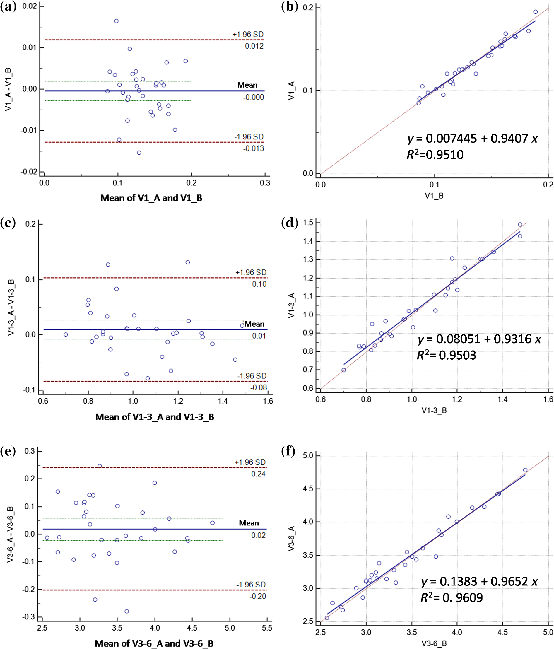
The mean and standard deviation of RVD, the CC, and $R^{2}$ of linear regression of the volumes obtained from repeated scans for the 1-mm center circle, 1- to 3-mm ring, and 3- to 6-mm ring, are shown in Table 2. High agreement can be observed. The RVD values are all smaller than 4%, the CC values are all larger than 0.97, and the $R^{2}$ values are all larger than 0.95. The Bland–Altman charts plotted in Fig. 6 also show that the difference between two groups of choroid volumes is small.

Table 2

Mean and standard deviation of relative choroid volume difference (RVD), CC, and coefficient of determination (R2) between repeated scans for 1-mm center circle, 1- to 3-mm ring, and 3- to 6-mm ring.

	1 mm	1 to 3 mm	3 to 6 mm
RVD (%)	$3.70 \pm 3.82$	$3.29 \pm 3.60$	$2.66 \pm 2.21$
CC	0.9752	0.9748	0.9803
$R^{2}$	0.9510	0.9503	0.9609

Fig. 6

The Bland–Altman charts and the linear regression charts for repeated volume quantifications: (a, b) for 1-mm center circle, (c, d) for 1- to 3-mm ring, and (e, f) for 3- to 6-mm ring.

3.2.

Qualitative Evaluation

Segmentation results overlaid on original B-scans are shown in Figs. 7 and 8 for two eyes, one with thick choroid and the other with thin choroid. Two B-scans with and without the fovea and ONH are shown for each eye. In the weak parts of CSI, as indicated by yellow arrows, both the difference between observers and the difference between automatic and manual segmentations are relatively higher. Compared with initialization results, the final segmentation is more close to the manual delineation.

Fig. 7

Segmentation results of an eye with thick choroid. Green and red curves refer to BM and CSI. Blue curves refer to the initialization of CSI. Yellow vertical lines refer to start and end of ONH. First column: original B-scans. Second and third columns: two manual segmentations. Fourth column: automatic results.

Fig. 8

Segmentation results of an eye with thin choroid. Green and red curves refer to BM and CSI. Blue curves refer to the initialization of CSI. Yellow vertical lines refer to start and end of ONH. First column: original B-scans. Second and third columns: two manual segmentations. Fourth column: automatic results.

Choroid thickness maps can be plotted according to automatic segmentation results. Six thickness maps of repeated scans from three eyes with large, medium, and small average choroid thickness are shown in Fig. 9. High resemblance can be observed from maps for the same eye, again proving the reproducibility of the proposed method.

Fig. 9

Choroid thickness maps obtained by automatic segmentation. The two columns correspond to results of repeated scans. The three rows correspond to three eyes with large, medium, and small choroid thickness.

3.3.

Comparison to Two-Dimensional Methods

As the existing methods were tested on different datasets with different scanning protocols and imaging resolutions, we are unable to compare with their results based on the reported errors. What is more, the intensity of RPE is usually the highest for EDI-OCT images, while not the case for SS-OCT images, and thus the BM segmentation for EDI-OCT images are not applicable for our dataset. Therefore, we only implemented and tested some 2-D CSI segmentation methods for comparison. As stated before, many methods designed for 2-D EDI-OCT images fail for our dataset with low SNR. For example, by Tian’s method,¹¹ the true CSI boundary points will be dominated by the “valley points” caused by noise. Because the method only uses location information but no intensity/gradient information in recovering the shortest path, the results will be much deviated from the true boundary. By Alonso-Caneiro et al.’s method,¹² the image enhancement essential for highlighting the CSI boundary will further magnify the noise, and thus results in very noisy cost functions. By Chen’s method,¹⁶ the gradual intensity distance below CSI will be corrupted by noise, as has been shown in Fig. 5(e). One feasible method is that of Ref. 15, designed for EDI-OCT B-scans with five times averaging, which have lower SNR. It is also a graph-based method but with different cost function. In testing, the same VOI undersegmented BM and excluding ONH is used for the searching of CSI. As tested, the 2-D method results in ABD of $22.02 \pm 4.81 μ m$ , which is statistically significantly larger than the proposed method ( $p < 0.0001$ ). The SBD is $13.86 \pm 7.50 μ m$ , indicating their results lie in some distance below the GT in general. Figure 10 shows the segmentation results in two consecutive B-scans. Notice that the 2-D method may be accurate in one B-scan, but not so in another. This is caused by the subtle difference between the two consecutive B-scans. While with our 3-D method, the segmentations are accurate in both B-scans, due to the constraints applied to 3-D neighbors.

Fig. 10

Comparison of CSI segmentation results with that of Ref. 15 for two consecutive B-scans. Cyan dotted curves refer to the results of proposed method. Yellow dashed curves refer to the results of Ref. 15. Blue solid curves refer to the GT. Yellow arrows point to the locations where the 2-D method results in errors due to variation between B-scans.

4. Conclusions

We have presented an automated 3-D choroid segmentation method for 1050-nm wide-view SS-OCT image volumes with low SNR. Effective methods for image quality enhancement and for ONH removal are proposed. Both gradient-based and region-based costs are used in the graph-based multiresolution method to detect the CSI with weak or broken boundaries. Using wavelet approximation, the gradual intensity distance measure originally proposed for high quality HD-OCT image segmentation is adopted to work successfully for SS-OCT images. The segmentation results are evaluated by comparison with manual segmentation and by a reproducibility test. The segmentation error is statistically significantly smaller than the interobserver variability. The reproducibility of volume quantification is high. Both quantitative and qualitative analyses show that the proposed method achieved good segmentation performance. Comparison to existing methods proves the superiority of the proposed method where 3-D context is considered. With the method, choroid thickness and volume both below the fovea and near the ONH can be quantitatively analyzed.

Currently the method is only tested on normal eyes. For eyes with pathology, several complications may add to the challenge of choroid segmentation. First, the RPE may be deformed, and relaxation of the smoothness constraint in graph search may be needed, as suggested in Ref. 24. Second, the CSI boundary may be further weakened. Other large lesions inside the retina and the choroid will also affect the segmentation accuracy. We will test the performance of the proposed method on pathological eyes and investigate the improvement in the future. Another limitation of the method lies in the detection of ONH. The termination in the upper boundary of photoreceptor/RPE complex is slightly different than the definition of neural canal opening (NCO), which is the termination of the RPE. By detecting the NCO, the ONH can be delineated more precisely, which will help both choroid segmentation nearby and other quantifications such as cup-disc ratio calculation.

Disclosures

The authors confirm that there are no competing interests.

Acknowledgments

This work has been supported by the National Basic Research Program of China (973 Program) under Grant No. 2014CB748600, the National Natural Science Foundation of China (NSFC) under Grants Nos. 81371629, 61401293, 61401294, 81401451, and 81401472, and the Natural Science Foundation of the Jiangsu Province under Grant No. BK20140052.

References

1.

D. L. Nickla and J. Wallman, “The multifunctional choroid,” Prog. Retinal Eye Res., 29 144 –168 (2010). http://dx.doi.org/10.1016/j.preteyeres.2009.12.002 PRTRES 1350-9462 Google Scholar

2.

X. Ding et al., “Choroidal thickness in healthy Chinese subjects,” Invest. Ophthalmol. Visual Sci., 52 9555 –9560 (2011). http://dx.doi.org/10.1167/iovs.11-8076 IOVSDA 0146-0404 Google Scholar

3.

V. Manjunath et al., “Choroidal thickness in normal eyes measured using Cirrus HD optical coherence tomography,” Am. J. Ophthalmol., 150 325 –329 (2010). http://dx.doi.org/10.1016/j.ajo.2010.04.018 AJOPAA 0002-9394 Google Scholar

4.

Z. Q. Yin et al., “Widespread choroidal insufficiency in primary open-angle glaucoma,” J. Glaucoma, 6 (1), 23 –32 (1997). http://dx.doi.org/10.1097/00061198-199702000-00006 JOGLES Google Scholar

5.

T. Fujiwara et al., “Enhanced depth imaging optical coherence tomography of the choroid in highly myopic eyes,” Am. J. Ophthalmol., 148 (3), 445 –450 (2009). http://dx.doi.org/10.1016/j.ajo.2009.04.029 AJOPAA 0002-9394 Google Scholar

6.

R. F. Spaide, “Age-related choroidal atrophy,” Am. J. Ophthalmol., 147 (5), 801 –810 (2009). http://dx.doi.org/10.1016/j.ajo.2008.12.010 AJOPAA 0002-9394 Google Scholar

7.

M. Gemenetzi, G. De Salvo and A. J. Lotery, “Central serous chorioretinopathy: an update on pathogenesis and treatment,” Eye, 24 (12), 1743 –1756 (2010). http://dx.doi.org/10.1038/eye.2010.130 Google Scholar

8.

I. Maruko et al., “Subfoveal choroidal thickness after treatment of Vogt-Koyanagi-Harada disease,” Retina, 31 (3), 510 –517 (2011). http://dx.doi.org/10.1097/IAE.0b013e3181eef053 RETIDX 0275-004X Google Scholar

9.

R. F. Spaide, H. Koizumi and M. C. Pozonni, “Enhanced depth imaging spectral-domain optical coherence tomography,” Am. J. Ophthalmol., 146 (4), 496 –500 (2008). http://dx.doi.org/10.1016/j.ajo.2008.05.032 AJOPAA 0002-9394 Google Scholar

10.

Y. Yasuno et al., “In vivo high-contrast imaging of deep posterior eye by

1 - μ m

swept source optical coherence tomography and scattering optical coherence angiography,” Opt. Express, 15 6121 –6139 (2007). http://dx.doi.org/10.1364/OE.15.006121 OPEXFF 1094-4087 Google Scholar

11.

J. Tian et al., “Automatic segmentation of the choroid in enhanced depth imaging optical coherence tomography images,” Biomed. Opt. Express, 4 (3), 397 –411 (2013). http://dx.doi.org/10.1364/BOE.4.000397 BOEICL 2156-7085 Google Scholar

12.

D. Alonso-Caneiro, S. A. Read and M. J. Collins, “Automatic segmentation of choroidal thickness in optical coherence tomography,” Biomed. Opt. Express, 4 (12), 2795 –2812 (2013). http://dx.doi.org/10.1364/BOE.4.002795 BOEICL 2156-7085 Google Scholar

13.

K. K. Vupparaboina et al., “Automated estimation of choroidal thickness distribution and volume based on OCT images of posterior visual section,” Comput. Med. Imaging Graphics, 46 (3), 315 –327 (2015). http://dx.doi.org/10.1016/j.compmedimag.2015.09.008 Google Scholar

14.

H. Danesh et al., “Segmentation of choroidal boundary in enhanced depth imaging OCTs using a multiresolution texture based modeling in graph cuts,” Comput. Math. Methods Med., 2014 479268 (2014). http://dx.doi.org/10.1155/2014/479268 Google Scholar

15.

Q. Chen et al., “Choroidal vasculature characteristics based choroid segmentation for enhanced depth imaging optical coherence tomography images,” Med. Phys., 43 1649 –1661 (2016). http://dx.doi.org/10.1118/1.4943382 Google Scholar

16.

Q. Chen et al., “Automated choroid segmentation based on gradual intensity distance in HD-OCT images,” Opt. Express, 23 (7), 8974 –8994 (2015). http://dx.doi.org/10.1364/OE.23.008974 OPEXFF 1094-4087 Google Scholar

17.

Z. Hu et al., “Semiautomated segmentation of the choroid in spectral-domain optical coherence tomography scans,” Invest. Ophthalmol. Visual Sci., 54 (3), 1722 –1729 (2013). http://dx.doi.org/10.1167/iovs.12-10578 IOVSDA 0146-0404 Google Scholar

18.

V. Kajic et al., “Automated choroidal segmentation of 1060 nm OCT in healthy and pathologic eyes using a statistical model,” Biomed. Opt. Express, 3 (1), 86 –103 (2012). http://dx.doi.org/10.1364/BOE.3.000086 BOEICL 2156-7085 Google Scholar

19.

L. Zhang et al., “Automated segmentation of the choroid from clinical SD-OCT,” Invest. Ophthalmol. Visual Sci., 53 (12), 7510 –7519 (2012). http://dx.doi.org/10.1167/iovs.12-10311 IOVSDA 0146-0404 Google Scholar

20.

A. Philip et al., “Choroidal thickness maps from spectral domain and swept source optical coherence tomography: algorithmic versus ground truth annotation,” Br. J. Ophthalmol., 100 (10), 1372 –1376 (2016). http://dx.doi.org/10.1136/bjophthalmol-2015-307985 BJOPAL 0007-1161 Google Scholar

21.

L. Zhang et al., “Validity of automated choroidal segmentation in SS-OCT and SD-OCT,” Invest. Ophthalmol. Visual Sci., 56 (5), 3202 –3211 (2015). http://dx.doi.org/10.1167/iovs.14-15669 IOVSDA 0146-0404 Google Scholar

22.

K. Mansouri et al., “Assessment of choroidal thickness and volume during water drinking test by swept-source optical coherence tomography,” Ophthalmology, 120 (12), 2508 –2516 (2013). http://dx.doi.org/10.1016/j.ophtha.2013.07.040 Google Scholar

23.

K. Mansouri et al., “Evaluation of retinal and choroidal thickness by swept-source optical coherence tomography: repeatability and assessment of artifacts,” Am. J. Ophthalmol., 157 (5), 1022 –1032 (2014). http://dx.doi.org/10.1016/j.ajo.2014.02.008 AJOPAA 0002-9394 Google Scholar

24.

F. Shi et al., “Automated 3-D retinal layer segmentation of macular optical coherence tomography images with serous pigment epithelial detachments,” IEEE Trans. Med. Imag., 34 (2), 441 –452 (2015). http://dx.doi.org/10.1109/TMI.2014.2359980 ITMID4 0278-0062 Google Scholar

25.

G. R. Wilkins, O. M. Houghton and A. L. Oldenburg, “Automated segmentation of intraretinal cystoid fluid in optical coherence tomography,” IEEE Trans. Biomed. Imag., 59 (4), 1109 –1114 (2012). http://dx.doi.org/10.1109/TBME.2012.2184759 Google Scholar

26.

C. Tomasi and R. Manduchi, “Bilateral filtering for gray and color images,” in Proc. IEEE Int. Conf. Computer Vision, 839 –846 (1998). http://dx.doi.org/10.1109/ICCV.1998.710815 Google Scholar

27.

S. Paris and F. Durand, “A fast approximation of the bilateral filter using a signal processing approach,” Int. J. Comput. Vision, 81 (1), 568 –580 (2006). http://dx.doi.org/10.1007/11744085_44 IJCVEQ 0920-5691 Google Scholar

28.

J. Canny, “A computational approach to edge detection,” IEEE Trans. Pattern Anal. Mach. Intell., PAMI-8 (6), 679 –698 (1986). http://dx.doi.org/10.1109/TPAMI.1986.4767851 ITPIDJ 0162-8828 Google Scholar

29.

K. Li et al., “Optimal surface segmentation in volumetric images—a graph-theoretic approach,” IEEE Trans. Pattern Anal. Mach. Intell., 28 (1), 119 –134 (2006). http://dx.doi.org/10.1109/TPAMI.2006.19 ITPIDJ 0162-8828 Google Scholar

30.

M. K. Garvin et al., “Automated 3-D intraretinal layer segmentation of macular spectral-domain optical coherence tomography images,” IEEE Trans. Med. Imag., 28 (9), 1436 –1447 (2009). http://dx.doi.org/10.1109/TMI.2009.2016958 ITMID4 0278-0062 Google Scholar

31.

Q. Song et al., “Optimal multiple surface segmentation with shape and context priors,” IEEE Trans. Med. Imag., 32 (2), 376 –386 (2013). http://dx.doi.org/10.1109/TMI.2012.2227120 ITMID4 0278-0062 Google Scholar

32.

X. Chen et al., “Three-dimensional segmentation of fluid-associated abnormalities in retinal OCT: probability constrained graph-search-graph-cut,” IEEE Trans. Med. Imag., 31 (8), 1521 –1531 (2012). http://dx.doi.org/10.1109/TMI.2012.2191302 ITMID4 0278-0062 Google Scholar

33.

P. A. Yushkevich et al., “User-guided 3D active contour segmentation of anatomical structures: significantly improved efficiency and reliability,” Neuroimage, 31 (3), 1116 –1128 (2006). http://dx.doi.org/10.1016/j.neuroimage.2006.01.015 NEIMEF 1053-8119 Google Scholar

34.

“Photocoagulation for diabetic macular edema. Early treatment diabetic retinopathy study report number 1,” Arch Ophthalmol., 103 1796 –1806 (1985). http://dx.doi.org/10.1001/archopht.1985.01050120030015 Google Scholar

Biography

Fei Shi is an assistant professor at Soochow University, Suzhou, China. She received her PhD in electrical engineering from Polytechnic University (now New York University Tandon School of Engineering), Brooklyn, United States, in 2006. She has coauthored over 20 papers in internationally recognized journals and conferences. Her current research is focused on medical image processing and analysis.

Xinjian Chen is a distinguished professor at Soochow University, Suzhou, China. He received his PhD from the Chinese Academy of Sciences in 2006. He conducted postdoctoral research at the University of Pennsylvania, National Institute of Health, and University of Iowa, USA, from 2008 to 2012. He has published over 80 top international journal and conference papers. He has also been granted with six patents.

Biographies for the other authors are not available.

Citation Download Citation

Fei Shi, Bei Tian, Weifang Zhu, Dehui Xiang, Lei Zhou, Haobo Xu, and Xinjian Chen "Automated choroid segmentation in three-dimensional 1-μm wide-view OCT images with gradient and regional costs," Journal of Biomedical Optics 21(12), 126017 (22 December 2016). https://doi.org/10.1117/1.JBO.21.12.126017

Received: 18 August 2016; Accepted: 2 December 2016; Published: 22 December 2016

Access the abstract

JOURNAL ARTICLE
11 PAGES

DOWNLOAD PAPER SAVE TO MY LIBRARY

GET CITATION

CITATIONS

Cited by 10 scholarly publications.

Explore citations on Lens.org

RIGHTS & PERMISSIONS

Get copyright permission Get copyright permission on Copyright Marketplace

KEYWORDS

Image segmentation

Optical coherence tomography

3D image processing

Wavelets

Signal to noise ratio

Image enhancement

Digital filtering

1.

Introduction