On the equivalence and differences between laser Doppler flowmetry and laser speckle contrast analysis

Ingemar Fredriksson; Marcus Larsson

doi:10.1117/1.JBO.21.12.126018

23 December 2016 On the equivalence and differences between laser Doppler flowmetry and laser speckle contrast analysis

Ingemar Fredriksson, Marcus Larsson

Author Affiliations +

Journal of Biomedical Optics, Vol. 21, Issue 12, 126018 (December 2016). https://doi.org/10.1117/1.JBO.21.12.126018

Abstract

Laser Doppler flowmetry (LDF) and laser speckle contrast analysis (LASCA) both utilize the spatiotemporal properties of laser speckle patterns to assess microcirculatory blood flow in tissue. Although the techniques analyze the speckle pattern differently, there is a close relationship between them. We present a theoretical overview describing how the LDF power spectrum and the LASCA contrast can be calculated from each other, and how both these can be calculated from an optical Doppler spectrum containing various degrees of Doppler shifted light. The theoretical relationships are further demonstrated using time-resolved speckle simulations. A wide range of Monte Carlo simulated tissue models is then used to show how perfusion estimates for LDF and LASCA are affected by changes in blood concentration and speed distribution, as well as by geometrical and optical properties. We conclude that perfusion estimates from conventional single exposure time LASCA are in general more sensitive to changes in optical and geometrical properties and are less accurate in the prediction of real perfusion changes, especially speed changes. Since there is a theoretical one-to-one relationship between Doppler power spectrum and contrast, one can conclude that those drawbacks with the LASCA technique can be overcome using a multiple exposure time setup.

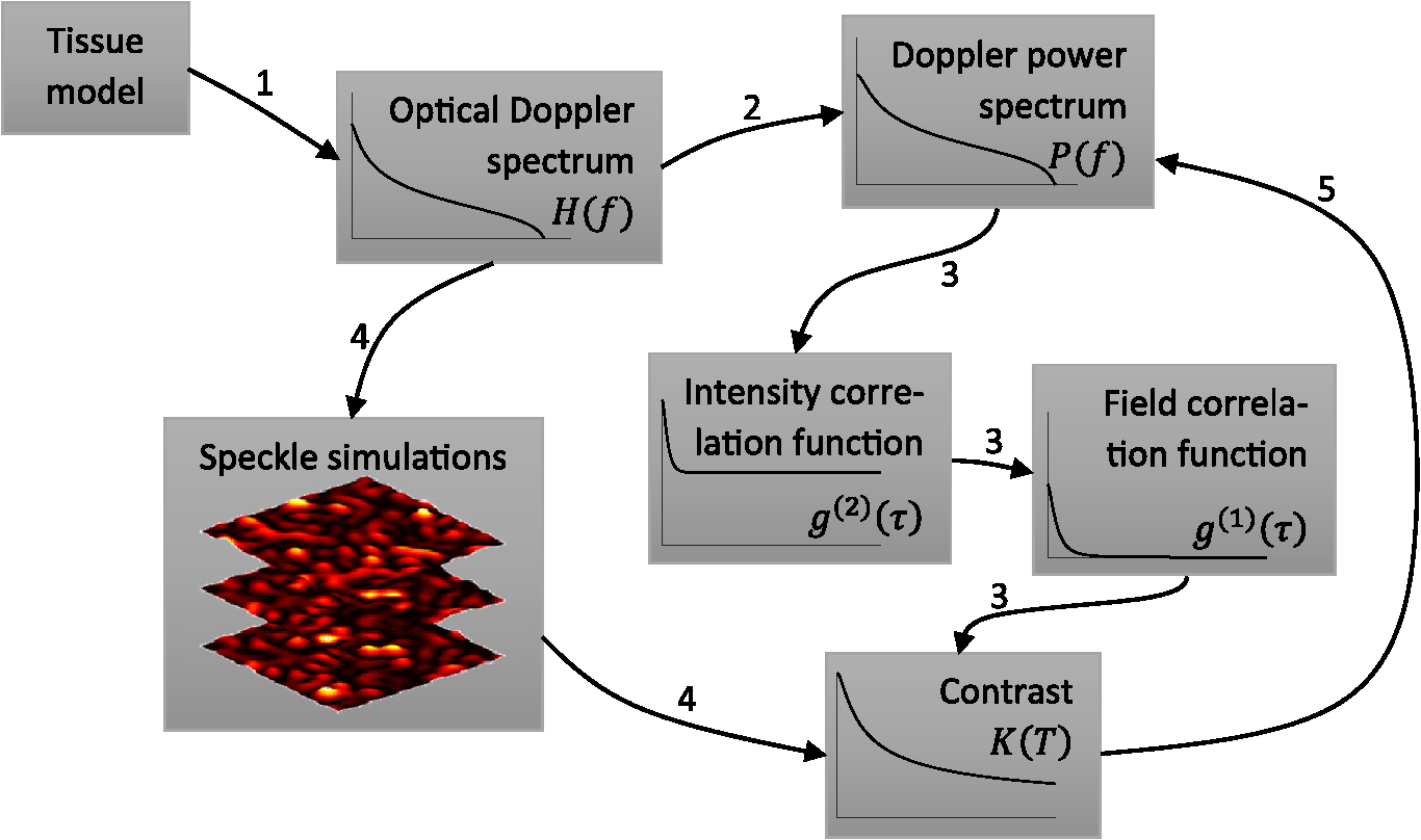
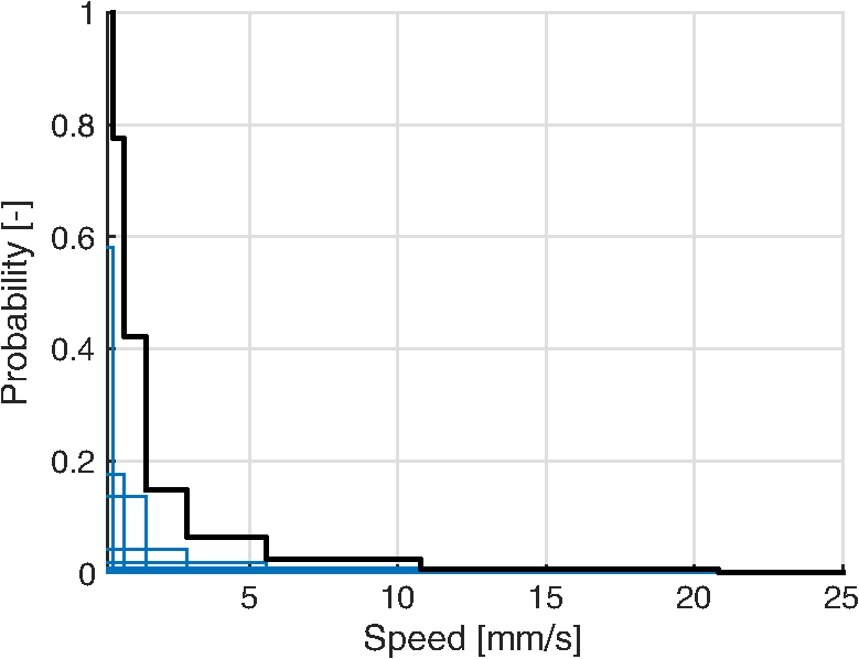
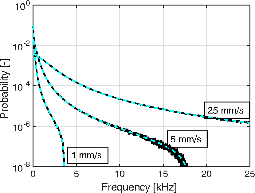
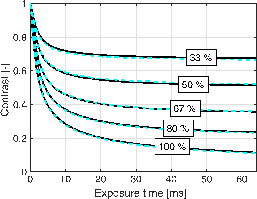
1. Introduction

In 1981, Fercher and Briers proposed and demonstrated that single exposure laser speckle images could be used to indirectly assess the microcirculatory blood flow by analyzing the local speckle contrast.¹ This technique, commonly referred to as laser speckle contrast analysis (LASCA) or laser speckle contrast imaging (LSCI), quantifies the magnitude of speckle movement by analyzing the spatial blurring that occurs as an effect of the Doppler shifts that are introduced when moving red blood cells scatter light. Since then the simplicity, usefulness, and applicability of the technique have been demonstrated in numerous medical studies.²^–⁵

An alternative way of quantifying the Doppler shifts is to study the temporal speckle fluctuations. In laser Doppler flowmetry (LDF), this is done by calculating the first moment of the Doppler power spectrum. It has been shown that this measure increases with both the speed and the amount of red blood cells.⁶^,⁷ Similar studies have experimentally shown that the LASCA technique displays comparable trends.⁸^–¹¹ However, for the LASCA technique, an additional dependency on the image exposure time is introduced.

The similarity between LASCA and LDF is further strengthened by the theory describing how the speckle contrast depends directly on the Doppler power spectrum¹² or the field correlation function.¹³ According to LDF theory, there is also a direct dependency among the field correlation function, the intensity correlation function, the optical Doppler spectrum (i.e., the histogram of Doppler frequencies), and the Doppler power spectrum.¹⁴^,¹⁵ Based on these relationships, Thompson and Andrews have demonstrated that the Doppler power spectrum can in fact be deduced from the speckle contrast if the contrast is resolved as a function of exposure time.¹⁶

In most LASCA studies, however, only a single exposure time has been used. As a single exposure LASCA image contains information from all Doppler frequencies, it will produce perfusion estimates that to some extent are sensitive to both the speed and the amount of moving red blood cells. Unlike the LDF approach, single exposure LASCA can only be used for studying the combined effect of speed and blood amount. How these two properties affect the speckle contrast is nontrivial and not yet fully explored, although some recent studies have focused on that.¹⁷^,¹⁸ Different ways of interpreting how the contrast is linked to the true tissue perfusion have been presented. Still the question of how well these proposed perfusion measures reflect the actual tissue perfusion remains unanswered. Furthermore, it is known that the optical and geometrical properties of the tissue under study affect the estimated perfusion value for both LDF and LASCA. How these properties affect the LDF-perfusion is known to some extent,¹⁹^,²⁰ whereas this is just beginning to be explored for LASCA.²¹

The aim of this article was to show how perfusion estimates calculated using LASCA depend on changes in blood flow speed distribution, blood tissue fraction, and optical properties and how they relate to the LDF-perfusion estimate. In order to do that, a comprehensive theoretical framework showing the relationship between LASCA and LDF is presented. This includes direct analytical forms to calculate the contrast as a function of exposure time from the Doppler power spectrum and vice versa and numerical methods for simulating both photon transport in tissue and the formation of dynamic speckle patterns on a detector.

2. Theory

The theory section is outlined in Fig. 1. It is described how the optical Doppler spectrum, i.e., the distribution of Doppler shifts, can be calculated from a tissue model (arrow 1). This is done either by assuming only single shifts with a certain speed of the red blood cells (RBC) (Sec. 2.1) or from a multilayered skin tissue model with certain geometrical and optical properties, blood concentration, and speed distribution (Sec. 2.2). The Doppler power spectrum is calculated as the autocorrelation of the optical Doppler spectrum (arrow 2).⁷ It is then shown how the contrast as a function of exposure time can be analytically calculated from the Doppler power spectrum via the intensity and field correlation functions (arrows 3, Sec. 2.3). For comparison, speckle simulations are run based on the optical Doppler spectrum, and the contrast is then calculated from the speckle simulations (arrows 4, Sec. 2.4). To close the loop, it is also described how the Doppler power spectrum can be analytically calculated from the contrast (arrow 5, Sec. 2.5).

Fig. 1

Overview of the steps covered in the theory section.

2.1.

Analytic Calculation of Single Shifted Optical Doppler Spectrum

When the scattering phase function of blood is represented by a Gegenbauer kernel phase function²² with the second parameter $α_{Gk} = 1$ , the histogram over single shifted Doppler frequencies RBC:s moving with speed $v$ can be expressed analytically. We have described this in an appendix to a previous paper,²³ but it is given again here for the consistency of this paper.

The Doppler frequency shift $f$ that results when light is scattered an angle $θ$ by an RBC moving with velocity $v$ can be expressed by

Eq. (1)

f = v \cdot q = \frac{2 n v}{λ} \sin (\frac{θ}{2}) \cos ϕ = \frac{2 n v}{λ} \sqrt{\frac{1 - \cos θ}{2}} \cos ϕ = [\begin{matrix} μ = \cos θ \\ ξ = \cos ϕ \end{matrix}] = \frac{2 n v}{λ} \sqrt{\frac{1 - μ}{2}} ξ,

where

v = | v |

,

q

is the difference between the incoming wave vector and the scattered wave vector,

λ

is the laser wavelength,

n

is the refractive index of the medium and

ϕ

is the angle between

v

and

q

. The single shifted optical Doppler spectrum for a given set of

v

,

λ

, and

n

can thus be calculated by considering the probability distributions of the angles

θ

and

ϕ

, where the latter can be assumed to be uniformly randomly distributed. Specifically, the probability to be calculated for each Doppler frequency

f

is the probability of

Eq. (2)

\sqrt{\frac{1 - μ}{2}} ξ = \frac{f λ}{\underset{A}{\underset{⏟}{2 n v}}} \Rightarrow \sqrt{\frac{1 - μ}{2}} = x and ξ = \frac{A}{x},

for all values of

x

between

A

and 1, i.e., for

μ \in [- 1, 1 - 2 A^{2}]

. The probability of

μ

is given by the scattering phase function of blood (Gegenbauer kernel with

g_{Gk} = 0.948

and

α_{Gk} = 1

, valid for 785 nm²⁴) and the probability of

ξ

can be assumed to be rectangular distributed between 0 and 1 for positive frequency shifts. The probability density function for

ξ = A / x

is given by

Eq. (3)

p_{ξ} (x) = \frac{A}{x} .

The probability density function for $μ$ is given by the scattering phase function (Gegenbauer kernel) which with $α = 1$ is

Eq. (4)

p_{μ} (μ) = \frac{K}{{(1 + g_{Gk}^{2} - 2 g_{Gk} μ)}^{2}}, where K = \frac{g_{Gk} {(1 - g_{Gk}^{2})}^{2}}{2 [{(1 + g_{Gk})}^{2} - {(1 - g_{Gk})}^{2}]} .

The probability density function, $p_{f} (f)$ for Doppler shift with frequency $f$ is thus calculated by

Eq. (5)

p_{f} (f) = \frac{1}{f} \int_{- 1}^{μ_{0}} p_{μ} (μ) p_{ξ} (\sqrt{\frac{1 - μ}{2}}) d μ = \dots = [B = \frac{{(1 - g_{Gk})}^{2}}{4 g_{Gk}}] = \frac{K λ}{8 n v g_{Gk}^{2}} \int_{A}^{1} \frac{1}{{(B + x^{2})}^{2}} d x = \frac{K λ}{\underset{a}{\underset{⏟}{2 n v g_{Gk} {(1 - g_{Gk})}^{2}}}} (\underset{b}{\underset{⏟}{\frac{1}{1 + B} + \frac{1}{\sqrt{B}} \arctan \frac{1}{\sqrt{B}}}} - \underset{c (f)}{\underset{⏟}{\frac{x}{A^{2} + B}}} - \underset{d (f)}{\underset{⏟}{\frac{1}{\sqrt{B}} \arctan \frac{A}{\sqrt{B}}}}) .

In practice, the probability for Doppler frequencies should rather be divided into a histogram, $H (f_{i})$ , with frequency bins $f_{i}$ to $f_{i + 1}$

Eq. (6)

H (f_{i}) = a \int_{f_{i}}^{f_{i + 1}} [b - c (f) - d (f)] d f = \frac{K λ}{2 n v g_{Gk} {(1 - g_{Gk})}^{2}} {[f (\frac{1}{1 + B} + \frac{1}{\sqrt{B}} \arctan \frac{1}{\sqrt{B}} - \frac{1}{\sqrt{B}} \arctan \frac{λ f}{2 n v \sqrt{B}})]}_{f_{i}}^{f_{i + 1}} .

Note that this expression is valid only for positive frequency shifts, but the shape is identical (mirrored) for negative frequency shifts.

The single shifted optical Doppler spectrum was also simulated by calculating Eq. (1) for a large number of random values for $\cos ϕ$ and $\cos θ$ . The values of $\cos ϕ$ were chosen from a rectangular distribution, whereas the values of $\cos θ$ (for $α_{Gk} = 1$ ) were chosen from Ref. 25

Eq. (7)

\cos θ = \frac{1}{2 g_{Gk}} {1 + g_{Gk}^{2} - {[ξ \frac{{(1 + g_{Gk})}^{2} - {(1 - g_{Gk})}^{2}}{{(1 - g_{Gk}^{2})}^{2}} + \frac{1}{{(1 + g_{Gk})}^{2}}]}^{- 1}},

where

ξ

is a random number between 0 and 1.

2.2.

From Tissue Model to Optical Doppler Spectrum

We have previously described the details of how an optical Doppler spectrum can be calculated for a given speed distribution from a multilayered biooptical model.²³^,²⁶ The method is based on path length distributions from Monte Carlo simulations from multilayered models with given geometries and scattering properties, where the effect of absorption is added using Beer–Lambert’s law. The optical Doppler spectrum is then calculated based on single shifted optical Doppler spectra [Eq. (6)] for each speed in the given speed distribution, which are multiple shifted with the number of shifts given by Poisson distributions that are based on the path length, the fraction of blood, and the scattering coefficient of blood.

In this study, Doppler power spectra were calculated in three layer models, with one bloodless epidermal layer containing melanin, and two dermis layers containing homogeneously distributed blood. The upper dermis layer had a thickness of 0.5 mm and the lower had a semi-infinite thickness, and the layers could contain different amounts of blood. For all models in this study, the refractive index in all layers was 1.4. The blood was modeled with an absorption coefficient of 0.58 and $0.38 {mm}^{- 1}$ for deoxygenized and oxygenized blood, respectively, a scattering coefficient of $222 {mm}^{- 1}$ , and a Gegenbauer kernel scattering phase function with $g_{Gk} = 0.948$ and $α_{Gk} = 1.0$ , resulting in an anisotropy factor of 0.991 and a reduced scattering coefficient of $2.0 {mm}^{- 1}$ . These values are valid for blood with 43% hematocrit, a hemoglobin value of $145 g Hb / L$ blood, and mean cell hemoglobin concentration of $345 g Hb / L$ RBC.²⁶ The optical properties are valid for 785 nm.

The base model used in Secs. 3.4 and 3.5 had an epidermal thickness of $75 μ m$ , a reduced scattering coefficient of all layers of $2.6 {mm}^{- 1}$ , and a melanin concentration of 1% (in the epidermis layer) with absorption coefficient of $15 {mm}^{- 1}$ . The blood tissue fraction was 1% in both dermis layers with an oxygen saturation of 80% and an average speed of $1 mm / s$ . In the random models in Sec. 3.6, all those parameters were randomly chosen.

The speed distribution in the model consisted of 10 rectangular distributions, each distributed between 0 and twice the average speed of that distribution. The average speeds were linearly distributed in the logarithmic plane from a minimum average speed, i.e., $v_{i} \in v_{\min} (1, 10^{v_{step}}, 10^{2 v_{step}}, \dots, 10^{9 v_{step}})$ , where $v_{\min} = 0.2 k$ and $v_{step} = 0.286$ , resulting in a maximum average speed of $75 k$ , where $k$ is a scaling factor. See Fig. 2 for an example of a speed distribution with $k = 1$ .

Fig. 2

Example of speed distribution in skin model. The probability of each rectangular distribution (blue, thin) sums up to the total probability distribution (black, thick). Note that the whole $x$ and $y$ scales are not shown ( $x$ reaches 150 and $y$ reaches about 2).

2.3.

From Doppler Power Spectrum to Contrast

The Doppler power spectrum $P (f)$ , i.e., the power spectral density of the temporal speckle intensity fluctuations, can be calculated for $f \neq 0$ using

Eq. (8)

P (f \neq 0) = H * H (f),

where

H (f)

is the optical Doppler spectrum and * denotes the cross correlation.⁷^,¹⁴ With this cross correlation, both homodyne and heterodyne mixing of shifted and unshifted E-fields are taken into account. In Eq. (8), it is assumed that

Eq. (9)

\int_{- \infty}^{\infty} H (f \neq 0) d f = f_{D},

where

f_{D}

is the fraction of Doppler shifted photons. For

f = 0

, the Doppler power is given by

Eq. (10)

P (f = 0) = \int_{- \infty}^{\infty} H (f) d f \cdot δ (f) = δ (f),

where

δ (f)

is the Dirac delta function. From the Doppler power spectrum, the intensity correlation function

g^{(2)}

can be calculated as

Eq. (11)

g^{(2)} (τ) = | F^{- 1} {P (f)} |,

where

F^{- 1}

is the inverse Fourier transform. Conventionally, the field correlation function

g^{(1)}

can be derived from the intensity correlation function using the Siegert relation. However, for light that has propagated through a nonergodic medium such as tissue, where only a fraction of the photons has been Doppler shifted, an extension of the Siegert relation is needed.¹⁵^,²⁷ This extension is given by

Eq. (12)

g^{(1)} (τ) = \sqrt{1 + g^{(2)} (τ) - g^{(2)} (0)} .

In a final step, the spatial speckle contrast $K$ can be calculated from the field correlation function using²⁸^,²⁹

Eq. (13)

K^{2} (T) = \frac{2 β}{T} \int_{0}^{T} {| g^{(1)} (τ) |}^{2} (1 - \frac{τ}{T}) d τ,

where

β

is the coherence factor that is treated by calibration measurements in practice, and

T

is the exposure time.

2.4.

Speckle Simulations

The intensity registered by a square-law imaging detector such as a CCD or CMOS sensor is described by

Eq. (14)

I = E E^{*},

where

E = \sum_{n} E_{n}

is the superpositioned E-field, consisting of both Doppler shifted and nonshifted E-fields. Each electromagnetic (EM) wave can be described by

Eq. (15)

E_{n} (r, t) = E_{0 n} e^{i (k r_{n} - (ω_{0} + Δ ω_{n}) t + φ_{n})} = E_{0 n} e^{- i ω_{0}} e^{i (k r_{n} - Δ ω_{n} t + φ_{n})},

where

E_{0 n}

is the wave amplitude,

k

the wave vector,

r_{n}

the position vector,

ω_{0}

the common carrier frequency (i.e., the laser frequency),

Δ ω_{n}

the Doppler frequency shift, and

φ_{n}

the initial phase of wave

n

. Combining Eqs. (14) and (15), gives

Eq. (16)

I (t) = (e^{- i ω_{0}} \sum_{n} E_{0 n} e^{- i ϕ_{n}}) (e^{i ω_{0}} \sum_{n} E_{0 n} e^{i ϕ_{n}}) = (\sum_{n} E_{0 n} e^{- i ϕ_{n}}) (\sum_{n} E_{0 n} e^{i ϕ_{n}}),

where

ϕ_{n} = k r_{n} - Δ ω_{n} t + φ_{n}

. Eq. (16) can be rewritten as

Eq. (17)

I (t) = {(\sum_{n} E_{0 n} \frac{e^{i ϕ_{n}}}{2} + \sum_{n} E_{0 n} \frac{e^{- i ϕ_{n}}}{2})}^{2} + {(\sum_{n} E_{0 n} \frac{e^{i ϕ_{n}}}{2 i} - \sum_{n} E_{0 n} \frac{e^{- i ϕ_{n}}}{2 i})}^{2} = {(\sum_{n} E_{0 n} \frac{e^{i ϕ_{n}} + e^{- i ϕ_{n}}}{2})}^{2} + {(\sum_{n} E_{0 n} \frac{e^{i ϕ_{n}} - e^{- i ϕ_{n}}}{2 i})}^{2} = {[\sum_{n} E_{0 n} \cos (ϕ_{n})]}^{2} + {[\sum_{n} E_{0 n} \sin (ϕ_{n})]}^{2} .

This equation implies that for a set of EM waves with known source position, amplitude, Doppler frequency, and initial phase, the intensity of the speckle pattern can be calculated at any position on a detector surface. By expanding Eqs. (15)–(17), the carrier frequency is dropped. This will remove the ill-conditioned numerical property of Eq. (15), where the carrier frequency is much larger than the Doppler frequency, enabling simulations to be run in single precision using GPUs for a massive computational speedup.

The simulated speckle patterns in this study have been generated using a total of 2000 Doppler shifted EM waves, each with a Doppler frequency ( $Δ ω_{n}$ ) that have been randomly picked from a predefined distribution given by the optical Doppler spectrum. In addition to those 2000 EM waves, 0 to 4000 non-Doppler shifted EM waves were used. Each EM wave was assigned a random initial phase (uniformly distributed at $[0, 2 π]$ ), simulating a fully developed speckle pattern. The position of the EM sources was randomly placed at a disc with a diameter 5 mm placed 50 mm away from the detector. The detector constituted 101 times 101 pixels, with a pixel pitch of $0.5 μ m$ . The development of each speckle pattern was simulated for 64 ms, with a time resolution of 0.02 ms, resulting in 3201 frames of speckle snapshots. The contrast for each speckle for different camera exposure times was calculated by adding consecutive snapshot frames. For each simulated exposure time $T$ , the speckle contrast was calculated as Ref. 30

Eq. (18)

K_{sim} (T) = \frac{σ (T)}{\bar{m}},

where

σ (T)

is the spatial standard deviation for exposure time

T

, and

\bar{m}

is the average intensity.

2.5.

From Contrast to Doppler Power Spectrum

For fully Doppler shifted speckle patterns, Thompson and Andrews¹⁶ have shown that the Doppler power spectrum can be calculated using the second derivative of the squared contrast with respect to the exposure time $T$ . Following their work, the second derivative of a partially Doppler shifted speckle pattern can be described by

Eq. (19)

\frac{d^{2}}{d T^{2}} [K^{2} (T) \frac{T^{2}}{2 β}] = \frac{d^{2}}{d T^{2}} [T \int_{0}^{T} {| g^{(1)} (τ) |}^{2} (1 - \frac{τ}{T}) d τ] = = \frac{d^{2}}{d T^{2}} {\int_{0}^{T} [1 + g^{(2)} (τ) - g^{(2)} (0)] (T - τ) d τ} = = \frac{d}{d T} [\int_{0}^{T} g^{(2)} (τ) d τ + T - T g^{(2)} (0)] = = g^{(2)} (τ) + 1 - g^{(2)} (0) .

The last term is given by Ref. 31

Eq. (20)

g^{(2)} (0) = 1 + f_{D}^{2} + 2 f (1 - f_{D}) = 1 + f_{D} (2 - f_{D}),

where

f_{D}

denotes the fraction of Doppler shifted light. Combining Eqs. (19) and (20) and applying the Fourier transform gives the Doppler power spectrum

Eq. (21)

P (f) = F {g^{(2)} (τ)} = F {\frac{d^{2}}{d T^{2}} [K^{2} (T) \frac{T^{2}}{2 β}] + f_{D} (2 - f_{D})},

where the last part of the above equation depends only on the fraction of Doppler shifted light while being independent of the exposure time

T

, and thus adds only to the zero frequency component of the power spectrum.

2.6.

Perfusion Estimates

In commercial LDF systems, the perfusion value is calculated from the first moment of the Doppler power spectrum, i.e.,

Eq. (22)

\int_{0}^{f_{\max}} f P (f) d f .

In commercial LASCA systems, the perfusion value is calculated from the contrast $K$ at one single exposure time, for example,⁵

Eq. (23)

\frac{1}{K} - 1

or

Eq. (24)

\frac{1}{K^{2}} - 1 .

If nothing else is stated, the perfusion estimates calculated using Eqs. (23) and (24) are calculated for contrasts for an exposure time of 6 ms.

3. Results

3.1.

Single Shifted Optical Doppler Spectrum

The analytic calculations of optical Doppler spectra, Eq. (6), were verified to simulations of one billion frequencies (see end of Sec. 2.1). The comparison, for three different speeds of the red blood cells, can be seen in Fig. 3.

Fig. 3

Comparison between simulated (solid) and analytically calculated (dashed) optical Doppler spectra for three different speeds.

3.2.

Comparison Between Simulated and Calculated Contrast

In order to verify the analytic expression to calculate contrast for various exposure times, the calculations were compared to contrast values calculated from speckle simulations. The optical Doppler spectra that the calculations and simulations were based on were calculated according to Eq. (6), with $v = 5 mm / s$ . The optical Doppler spectra were calculated for $2^{13}$ frequency bins distributed between $- 25$ and 25 kHz. From each of the resulting optical Doppler spectra, 2000 unique frequencies were randomly chosen. In addition, 0 to 4000 zero frequencies were added, giving fractions of Doppler shifted light, $f_{D}$ , of 33% to 100%. Contrast values for various exposure times were calculated based on the chosen frequencies according to Eqs. (8)–(13). For the same chosen frequencies, speckle simulations were performed for time instances 0, 0.02, 0.04, …, 64 ms. Contrast was then calculated from those speckle simulations by averaging data from consecutive time instances over a length corresponding to the required exposure time.

The results of the analytically calculated and simulated contrasts are shown in Fig. 4. Note that the contrast approaches $1 - f_{D}$ for long exposure times, which has been shown by Ragol et al.³²

Fig. 4

Comparison between contrast curves analytically calculated (solid) and simulated (dashed). Curves for 33% to 100% Doppler shifted light are shown.

3.3.

Contrast to Doppler Power Spectrum

In Fig. 5, a comparison between original Doppler power spectra and spectra that are first calculated to contrast [Eqs. (8)–(13)] and then recalculated to Doppler power spectra [Eq. (21)] is presented. The original spectra were for three different speeds (1, 5, and $25 mm / s$ , respectively), all with 80% Doppler shifted light. The Doppler power spectra were calculated for $2^{13}$ frequency bins between $- 25$ and 25 kHz, resulting in exposure times between 0 and 82 ms, with steps of 0.02 ms.

Fig. 5

Comparison between original Doppler power spectra (solid) and power spectra calculated from contrast decline curves (dashed) for two different speeds.

In practice, it is hardly realistic to achieve images with exposure times in steps of 0.02 ms with today’s cameras. Something that could be possible to achieve is contrast from exposure times with 1 ms steps, i.e., 1, 2, 3, … ms exposure times. In order to calculate a Doppler power spectrum with frequencies above 1 kHz from contrasts with only those exposure times, the contrasts for intermediate exposure times, including exposure times below 1 ms, have to be interpolated. In Fig. 6(a), the contrast that is interpolated from the points 0, 1, … 82 ms is compared to the original, high-resolution contrast. A logarithmic time scale is used in the plot where it is apparent that there are deviations between the interpolated and the original contrasts foremost between 0 and 1 ms. When calculating the Doppler power spectrum from those two contrast curves, it is apparent that especially frequencies above 1 kHz become highly distorted [Fig. 6(b)]. In this example, the original optical Doppler spectrum was based on single shifts with RBC speed of $5 mm / s$ , 80% Doppler shifted light. A shape-preserving piecewise cubic interpolation (MATLAB) was used. The resulting perfusion estimates [Eq. (22)], which were calculated from the Doppler power spectra in Fig. 6(b), were 242 and 527, respectively.

Fig. 6

(a) Contrast curve from single shifted optical Doppler spectrum with RBC speed $5 mm / s$ , 80% Doppler shifted light (solid), and contrast curve interpolated from the original curve in the points 0, 1, …, 82 ms using a shape-preserving piecewise cubic interpolation (dashed). (b) Doppler power spectra calculated from original (solid) and interpolated (dashed, noisy-looking) contrast curves.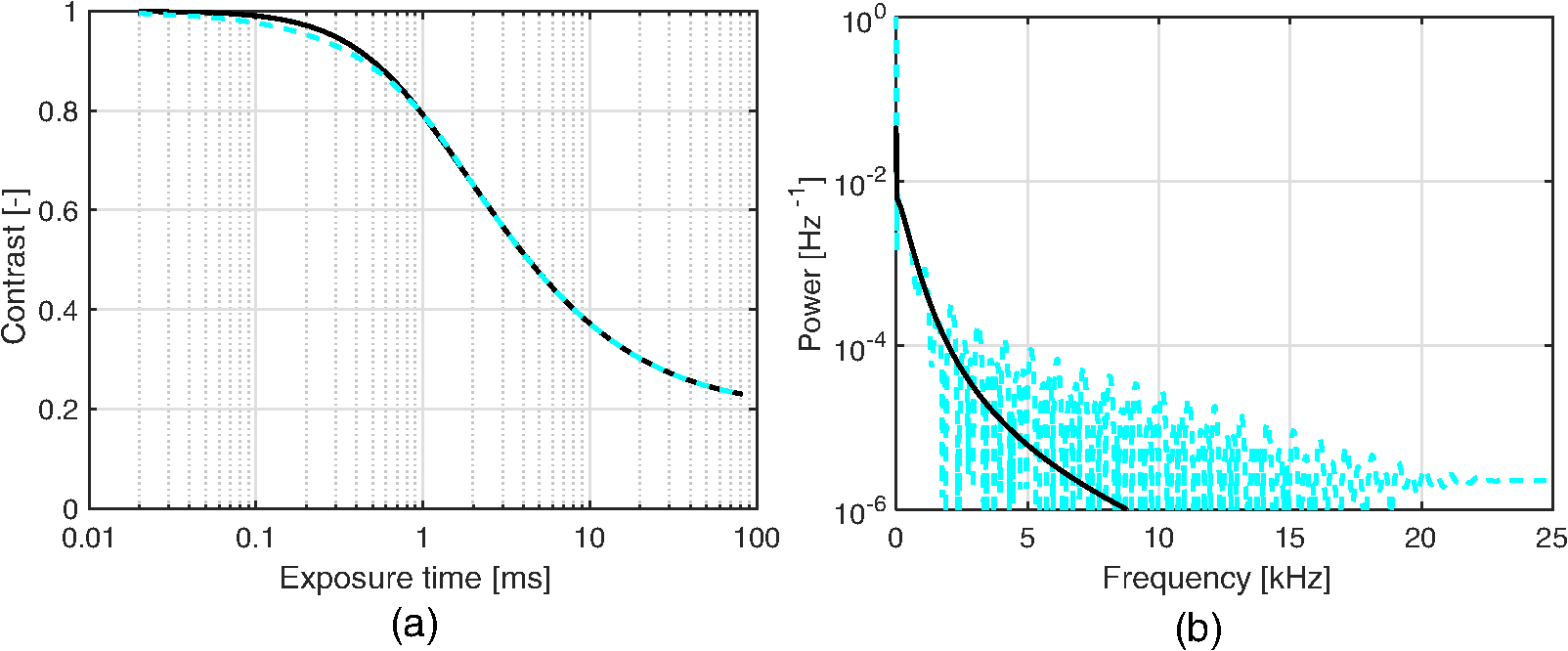

3.4.

Blood Perfusion Effect on Contrast

It was investigated how speed distribution and blood tissue fraction affect the contrast and the LASCA-perfusion estimate calculated with Eq. (24). In order to do that, optical Doppler spectra were calculated from a skin model as described in Sec. 2.2. The effect of changed blood tissue fraction is visualized in Fig. 7, whereas the effect of blood flow speed is visualized in Fig. 8. The LASCA-perfusion is normalized with the average perfusion for each exposure time in each plot.

Fig. 7

The effect on contrast (a and b) and perfusion (c and d) when changing the blood tissue fraction for two different average speeds: $0.2 mm / s$ (a and c) and $1.0 mm / s$ (b and d). Perfusions were normalized with average for each curve in c and d.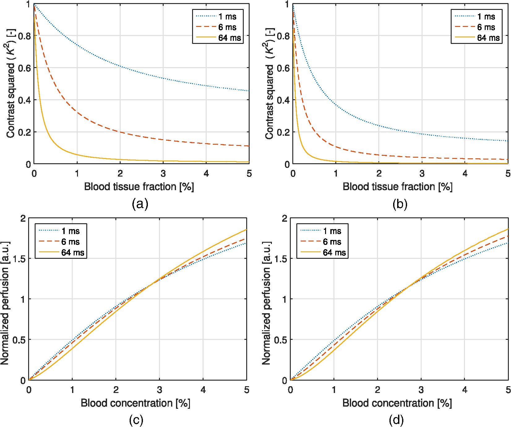

Fig. 8

The effect on contrast (a and b) and LASCA-perfusion (c and d) when changing the average blood flow speed for two different blood tissue fractions; 0.2% (a and c) and 1.0% (b and d). Two different speed distributions were used, the distribution described in Sec. 2.2 (thick) and a rectangular distribution between 0 and twice the speed on the $x$ -axis (thin). Perfusions were normalized with average for each curve in c and d.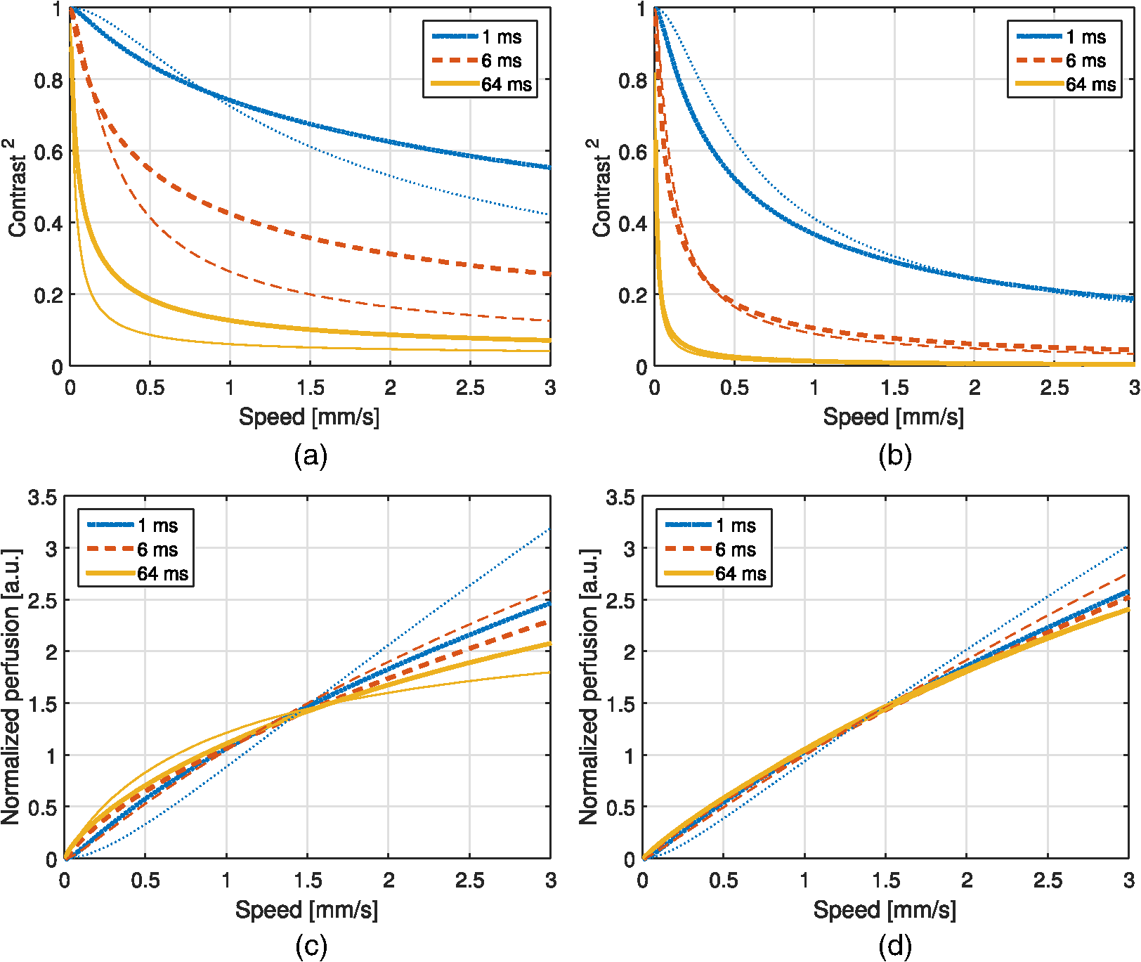

3.5.

Effect of Geometrical and Optical Properties

The size of each single Doppler shift is directly dependent on the scattering angle, and thus the scattering phase function of blood.⁷ It is therefore expected that the Doppler power spectrum and the contrast are affected by changing that parameter. The effect on the perfusion estimates when changing the anisotropy factor $g$ from the original value is summarized in Table 1. This was done both for a constant scattering coefficient $μ_{s} = 222 {mm}^{- 1}$ so that the reduced scattering coefficient $μ_{s}^{'}$ was affected, and by also changing $μ_{s}$ so that $μ_{s}^{'}$ was kept constant at $2.0 {mm}^{- 1}$ .

Table 1

Effect on LDF- and LASCA-perfusion estimates when changing scattering properties of blood, normalized to first line.

Blood scattering properties			Normalized perfusion estimates [-]
g (-)	μs (mm−1)	μs′ (mm−1)	LDF-perf	1/K−1	1/K2−1
0.991	222	2.0	1.00	1.00	1.00
0.987	222	2.9	1.20	1.17	1.21
0.980	222	4.4	1.54	1.39	1.48
0.970	222	6.7	1.92	1.63	1.81
0.987	154	2.0	0.92	0.81	0.78
0.980	100	2.0	0.86	0.60	0.56
0.970	67	2.0	0.79	0.46	0.42

When changing the reduced scattering coefficient of the static medium, the perfusion reached a maximum for values of about $2 {mm}^{- 1}$ . The relative change was highest for the longest exposure time. The effect is summarized in Table 2.

Table 2

Effect of changed scattering properties of the static medium. Perfusion estimates are normalized to the level at μs′=2.0 mm−1.

μs′ (mm−1)	LDF-perf	1/K−1	1/K2−1
1.0	0.93	0.98	0.97
2.0	1.0	1.0	1.0
5.0	0.95	0.82	0.75
10	0.82	0.61	0.48

Changing the thickness of the epidermis layer has an effect on the fraction of Doppler shifted photons, which in turn affect the contrast and perfusion estimates. The effect is summarized in Table 3.

Table 3

Effect of epidermis thickness on fraction of Doppler shifted light (fD) and perfusion estimates. Perfusion estimates are normalized to thickness of 0 mm.

Thickness (mm)	fD (-)	LDF-perf	1/K−1	1/K2−1
0	0.76	1.0	1.0	1.0
0.1	0.74	0.93	0.88	0.91
0.3	0.71	0.88	0.78	0.83
0.5	0.66	0.83	0.68	0.74

Finally, the melanin content in the skin also has a small effect on the perfusion estimates. The perfusion decreased with less than 15% when changing the melanin content from 0% to 40% except for 40% melanin concentration in $360 - μ m$ -thick epidermis layer. Such high melanin concentration in such thick epidermis is hardly realistic. The effect was much higher for the LASCA-perfusion estimates and higher for thicker epidermis layer (higher total amount of melanin). The results are summarized in Table 4.

Table 4

Effect of melanin concentration on perfusion estimates for two different epidermis thicknesses (tEpi). Perfusion estimates are normalized to the melanin concentration of 0% for each of the two thicknesses.

tEpi (μm)	Melanin conc. (%)	LDF-perf	1/K−1	1/K2−1
75	0	1.0	1.0	1.0
	2.5	1.0	1.0	0.99
	10	0.99	0.99	0.98
	40	0.99	0.97	0.96
360	0	1.0	1.0	1.0
	2.5	0.99	0.97	0.95
	10	0.96	0.90	0.85
	40	0.58	0.32	0.22

3.6.

Perfusion Predictability

Based on the skin model described in Sec. 2.2, 2000 random models with varied blood concentration, speed distribution, optical properties of static media, and geometries were generated. The true perfusion in the models, i.e., the actual RBC tissue fraction times their average speed, was calculated resulting in the perfusion unit [% $RBC \times mm / s$ ]. The optical Doppler spectrum and Doppler power spectrum were calculated, and the LDF-perfusion was calculated from the power spectrum [Eq. (22)]. In addition, the contrast was calculated from the power spectrum and the LASCA-perfusion was calculated from the contrast, based on both Eqs. (23) and (24). In Fig. 9, the LDF- and LASCA-perfusions are plotted against the true perfusion. The LDF- and LASCA-perfusions are normalized at 0.05% $RBC \times mm / s$ . Data were sorted with respect to the true perfusion and divided into groups with 100 models in each group, from which average values and standard deviations were calculated and plotted.

Fig. 9

Estimated LDF-perfusion from original Doppler power spectrum calculated with Eq. (22) and LASCA-perfusions calculated with either Eqs. (23) or (24). The data points represent average estimated perfusion in each group of 100 models, with the error bars showing the standard deviation.

It was also studied how the perfusion estimates were affected by isolated changes in average speed or RBC tissue fraction. In order to do that, the same 2000 models as above were used, and in each of the models either the average speed was increased by 10% or the RBC tissue fraction was increased by 10%. Both these changes would ideally generate a 10% increase in the resulting perfusion estimates. The actual response in the three calculated perfusion estimates is shown in Fig. 10. Data were sorted with respect to either average speed (a) or RBC tissue fraction (b) and divided into groups with 100 models in each group, from which average values and standard deviations were calculated. The average (standard deviation) estimated perfusion increase was 9.7 (0.2)%, 5.9 (0.9)%, and 8.1 (0.9)%, respectively, for LDF-perfusion, and the LASCA-perfusions calculated with $1 / K - 1$ [Eq. (23)] and $1 / K^{2} - 1$ [Eq. (24)] when average speed was increased 10%. Corresponding numbers when RBC tissue fraction was increased 10% were 6.6 (1.2)%, 7.3 (1.6)%, and 10 (1.5)%. The average standard deviation for the groups shown in Fig. 10 was 0.12%, 0.58%, and 0.85%, respectively, for the three perfusion estimates when average speed was increased 10%. Corresponding numbers when RBC tissue fraction was increased 10% were 0.36%, 0.62%, and 0.92%.

Fig. 10

Relative change in perfusion when (a) the average speed was increased 10% and (b) when the average RBC tissue fraction was increased 10%. The data points represent average response in each group of 100 models, with the error bars showing the standard deviation.

4. Discussion

We have described how the contrast can be calculated from the optical Doppler spectrum, via the Doppler power spectrum, and vice versa. Together with the generation of optical Doppler spectra from relevant tissue models, this can be used as a toolbox for further studies on the LASCA technique for a deeper understanding and, potentially, development of better blood perfusion measures.

It is shown in Fig. 3 that the single shifted optical Doppler spectrum can be calculated analytically for a given speed distribution and scattering phase function in an accurate and effective manner.

The results in Fig. 4 clearly show that the analytically calculated contrast values agree with the simulated contrast values. The small differences seen, with no particular trends, most likely originate from the fact that the simulations were based on a limited number of light sources randomly distributed over an area. Increasing the number of random points decreases the differences, but as these simulations are rather time consuming, they were limited to a maximum of 6000 points in this study. It should also be noted that it is important to have small time steps in the speckle simulations for correct results. For example, for correct contrast values at 0.5 ms exposure time, the time step had to be $\sim 0.02 ms$ or smaller.

When calculating the Doppler power spectrum from the contrast as in Fig. 5, the first- and second-order derivatives of $K^{2}$ are numerically estimated. For short exposure times, that estimation is not exact, which explains the small difference seen in Fig. 5 for especially the highest speed. The effect is pushed toward higher frequencies when increasing the sampling rate, i.e., decreasing the time steps in the contrast curve. Although we show that it is theoretically possible to calculate the Doppler power spectrum from the contrast curve, it is probably not the best way to go in order to calculate the best possible perfusion estimate. The results in Fig. 6 show that the Doppler power spectrum becomes highly distorted when calculating it from a contrast curve containing interpolated new contrast values from the original contrast values taken at realistic multiple exposure times. Maybe the interpolation can be improved in order to keep a continuous first- and second-order derivative, thus avoiding the overtones in the Doppler power spectrum, but even then, it is a computationally demanding way to go.

Studying the results in Figs. 7 and 8 gives some fundamental insights about the effect on contrast when changing blood flow parameters in a typical case. First, those figures reveal that the contrast and thus the LASCA-perfusion is sensitive to blood concentrations and flow speeds over a wide range. Another interesting finding is that the contrast is sensitive to the shape of the speed distribution, not only to the average speed, and nonlinearities arise at different speeds depending on that shape. This is in line with the findings by Ramirez-San-Juan et al.³³ Furthermore, the nonlinearities of perfusion in respect to speed depend on the blood concentration, as seen when comparing Figs. 8(c) and 8(d), where a lower blood concentration results in more severe nonlinearities in that particular example. The results are in line with a recent publication by Khaksari and Kirkpatrick,¹⁸ where the LASCA-perfusion is studied in more detail in terms of diffusive and advective flux.

We have compared two common alternative equations for calculating a perfusion estimate based on a single exposure time, Eqs. (23) and (24). In Fig. 9, it can be seen that the latter has a more linear relationship with the true perfusion, whereas the former resembles the LDF-perfusion more closely. In most of the presented results, an exposure time of 6 ms has been used. We have observed that most trends, for example, the effect of changing optical properties, are similar for other exposure times as well, but the effects are generally smaller for shorter exposure times. Furthermore, when changing optical and geometrical properties in the model, the LASCA-perfusion estimates are more affected than the LDF-perfusion estimate, see, for example, Tables 1–4.

The results in Fig. 10 are interesting and important since these techniques are often used to study relative changes in perfusion spatially and/or temporally. It can be seen that the LDF-perfusion estimate responds better to changes in average speed than either LASCA estimate. The increase in the estimated LDF-perfusion responds almost perfectly to the increase in speed in the models. This is not surprising as the LDF-perfusion, in contrast to the LASCA-perfusion, scales linearly to changes in Doppler frequencies, which directly depend on the speed of the moving scatterers. The response in the LASCA-perfusion estimates on the other hand is generally too low and is somewhat dependent on the level of the average speed (i.e., nonlinear) and is less predictable (much higher standard deviations). For changes in RBC tissue fraction, it can be seen that all perfusion estimates are nonlinear, i.e., the response is generally smaller for models with higher RBC tissue fraction. As for an increased average speed, the response for an increased RBC tissue fraction is less predictable with the LASCA-perfusion estimates. In all cases, the response for the perfusion estimate calculated with Eq. (24), i.e., $1 / K^{2} - 1$ , is stronger than the response calculated with Eq. (23), i.e., $1 / K - 1$ , which was expected.

This article has shown that there is a direct relationship between the Doppler power spectrum and the speckle contrast as a function of exposure time, utilized in LDF and LASCA, respectively. Due to practical limitations, commercially available LASCA systems use only a single exposure time when calculating the perfusion estimate. This data reduction results in a less predictable perfusion estimate than for LDF. In order to improve the perfusion estimate given by the LASCA technique at least to the level of the conventional LDF-perfusion estimate, a multiple exposure time LASCA has to be employed.³⁴^,³⁵

Disclosures

No conflicts of interest, financial or otherwise, are declared by the authors.

Acknowledgments

This study was financially supported by the Swedish Research Council (grant no. 2014-6141) and by the CENIIT research organization within Linköping University (project id. 11.02).

References

1.

A. F. Fercher and J. D. Briers, “Flow visualization by means of single-exposure speckle photography,” Opt. Commun., 37 (5), 326 –330 (1981). http://dx.doi.org/10.1016/0030-4018(81)90428-4 OPCOB8 0030-4018 Google Scholar

2.

F. Lindahl, E. Tesselaar and F. Sjöberg, “Assessing paediatric scald injuries using laser speckle contrast imaging,” Burns, 39 (4), 662 –666 (2013). http://dx.doi.org/10.1016/j.burns.2012.09.018 BURND8 0305-4179 Google Scholar

3.

M. Roustit and J. L. Cracowski, “Assessment of endothelial and neurovascular function in human skin microcirculation,” Trends Pharmacol. Sci., 34 (7), 373 –384 (2013). http://dx.doi.org/10.1016/j.tips.2013.05.007 Google Scholar

4.

B. Ruaro et al., “Laser speckle contrast analysis: a new method to evaluate peripheral blood perfusion in systemic sclerosis patients,” Ann. Rheum. Dis., 73 (6), 1181 –1185 (2014). http://dx.doi.org/10.1136/annrheumdis-2013-203514 Google Scholar

5.

D. Briers et al., “Laser speckle contrast imaging: theoretical and practical limitations,” J. Biomed. Opt., 18 (6), 066018 (2013). http://dx.doi.org/10.1117/1.JBO.18.6.066018 JBOPFO 1083-3668 Google Scholar

6.

G. E. Nilsson, “Signal processor for laser Doppler tissue flowmeters,” Med. Biol. Eng. Comput., 22 (4), 343 –348 (1984). http://dx.doi.org/10.1007/BF02442104 MBECDY 0140-0118 Google Scholar

7.

I. Fredriksson, M. Larsson, T. Strömberg, “Laser Doppler flowmetry,” Microcirculation Imaging, 67 –86 Wiley-Blackwell, Weinheim, Germany (2012). Google Scholar

8.

K. R. Forrester et al., “Comparison of laser speckle and laser Doppler perfusion imaging: measurement in human skin and rabbit articular tissue,” Med. Biol. Eng. Comput., 40 (6), 687 –697 (2002). http://dx.doi.org/10.1007/BF02345307 MBECDY 0140-0118 Google Scholar

9.

K. R. Forrester et al., “A laser speckle imaging technique for measuring tissue perfusion,” IEEE Trans. Biomed. Eng., 51 (11), 2074 –2084 (2004). http://dx.doi.org/10.1109/TBME.2004.834259 IEBEAX 0018-9294 Google Scholar

10.

C. Millet et al., “Comparison between laser speckle contrast imaging and laser Doppler imaging to assess skin blood flow in humans,” Microvasc. Res., 82 (2), 147 –151 (2011). http://dx.doi.org/10.1016/j.mvr.2011.06.006 MIVRA6 0026-2862 Google Scholar

11.

S. Sun et al., “Comparison of laser Doppler and laser speckle contrast imaging using a concurrent processing system,” Opt. Lasers Eng., 83 1 –9 (2016). http://dx.doi.org/10.1016/j.optlaseng.2016.02.021 OLENDN 0143-8166 Google Scholar

12.

M. J. Draijer et al., “Relation between the contrast in time integrated dynamic speckle patterns and the power spectral density of their temporal intensity fluctuations,” Opt. Express, 18 (21), 21883 –21891 (2010). http://dx.doi.org/10.1364/OE.18.021883 OPEXFF 1094-4087 Google Scholar

13.

D. A. Boas and A. G. Yodh, “Spatially varying dynamical properties of turbid media probed with diffusing temporal light correlation,” J. Opt. Soc. Am. A, 14 (1), 192 –215 (1997). http://dx.doi.org/10.1364/JOSAA.14.000192 Google Scholar

14.

A. T. Forrester, “Photoelectric mixing as a spectroscopic tool,” J. Opt. Soc. Am., 51 (3), 253 –259 (1961). http://dx.doi.org/10.1364/JOSA.51.000253 JOSAAH 0030-3941 Google Scholar

15.

H. Furukawa and S. Hirotsu, “Dynamic light scattering from static and dynamic fluctuations in inhomogeneous media,” J. Phys. Soc. Jpn., 71 (12), 2873 –2880 (2002). http://dx.doi.org/10.1143/JPSJ.71.2873 JUPSAU 0031-9015 Google Scholar

16.

O. B. Thompson and M. K. Andrews, “Tissue perfusion measurements: multiple-exposure laser speckle analysis generates laser Doppler-like spectra,” J. Biomed. Opt., 15 (2), 027015 (2010). http://dx.doi.org/10.1117/1.3400721 JBOPFO 1083-3668 Google Scholar

17.

S. M. Kazmi et al., “Flux or speed? Examining speckle contrast imaging of vascular flows,” Biomed. Opt. Express, 6 (7), 2588 –2608 (2015). http://dx.doi.org/10.1364/BOE.6.002588 Google Scholar

18.

K. Khaksari and S. J. Kirkpatrick, “Laser speckle contrast imaging is sensitive to advective flux,” J. Biomed. Opt., 21 (7), 076001 (2016). http://dx.doi.org/10.1117/1.JBO.21.7.076001 JBOPFO 1083-3668 Google Scholar

19.

M. Larsson, W. Steenbergen and T. Strömberg, “Influence of optical properties and fiber separation on laser Doppler flowmetry,” J. Biomed. Opt., 7 (2), 236 –243 (2002). http://dx.doi.org/10.1117/1.1463049 JBOPFO 1083-3668 Google Scholar

20.

I. Fredriksson, M. Larsson, T. Strömberg, “Model-based quantification of skin microcirculatory perfusion,” Computational Biophysics of the Skin, 395 –418 Pan Stanford Publishing, Singapore (2014). Google Scholar

21.

K. Khaksari and S. J. Kirkpatrick, “Combined effects of scattering and absorption on laser speckle contrast imaging,” J. Biomed. Opt., 21 (7), 076002 (2016). http://dx.doi.org/10.1117/1.JBO.21.7.076002 JBOPFO 1083-3668 Google Scholar

22.

L. O. Reynolds and N. J. McCormick, “Approximate two-parameter phase function for light scattering,” J. Opt. Soc. Am., 70 (10), 1206 –1212 (1980). http://dx.doi.org/10.1364/JOSA.70.001206 JOSAAH 0030-3941 Google Scholar

23.

I. Fredriksson et al., “Inverse Monte Carlo in a multilayered tissue model: merging diffuse reflectance spectroscopy and laser Doppler flowmetry,” J. Biomed. Opt., 18 (12), 127004 (2013). http://dx.doi.org/10.1117/1.JBO.18.12.127004 JBOPFO 1083-3668 Google Scholar

24.

I. Fredriksson, M. Larsson and T. Strömberg, “Optical microcirculatory skin model: assessed by Monte Carlo simulations paired with in vivo laser Doppler flowmetry,” J. Biomed. Opt., 13 (1), 014015 (2008). http://dx.doi.org/10.1117/1.2854691 JBOPFO 1083-3668 Google Scholar

25.

J. Swartling, “Biomedical and atmospheric applications of optical spectroscopy in scattering media,” Lund Reports on Atomic Physics, 290 113 Lund University, Lund (2002). Google Scholar

26.

I. Fredriksson, M. Larsson and T. Strömberg, “Model-based quantitative laser Doppler flowmetry in skin,” J. Biomed. Opt., 15 (5), 057002 (2010). http://dx.doi.org/10.1117/1.3484746 JBOPFO 1083-3668 Google Scholar

27.

P. N. Pusey and W. van Megen, “Dynamic light scattering by non-ergodic media,” Phys. A, 157 (2), 705 –741 (1989). http://dx.doi.org/10.1016/0378-4371(89)90063-0 Google Scholar

28.

K. Schatzel, “Noise on photon correlation data. I. Autocorrelation functions,” Quantum Opt., 2 (4), 287 (1990). http://dx.doi.org/10.1088/0954-8998/2/4/002 QUOPET 0954-8998 Google Scholar

29.

P. Zakharov et al., “Quantitative modeling of laser speckle imaging,” Opt. Lett., 31 (23), 3465 –3467 (2006). http://dx.doi.org/10.1364/OL.31.003465 OPLEDP 0146-9592 Google Scholar

30.

J. D. Briers and G. J. Richards, “Laser speckle contrast analysis (LASCA) for flow measurement,” Optical Inspection and Micromeasurements II, SPIE, Munich, Germany (1997). Google Scholar

31.

A. B. Parthasarathy et al., “Robust flow measurement with multi-exposure speckle imaging,” Opt. Express, 16 (3), 1975 –1989 (2008). http://dx.doi.org/10.1364/OE.16.001975 OPEXFF 1094-4087 Google Scholar

32.

S. Ragol et al., “Static laser speckle contrast analysis for noninvasive burn diagnosis using a camera-phone imager,” J. Biomed. Opt., 20 (8), 086009 (2015). http://dx.doi.org/10.1117/1.JBO.20.8.086009 JBOPFO 1083-3668 Google Scholar

33.

J. C. Ramirez-San-Juan, J. S. Nelson and B. Choi, “Comparison of Lorentzian and Gaussian based approaches for laser speckle imaging of blood flow dynamics,” Proc. SPIE, 6079 607924 (2006). http://dx.doi.org/10.1117/12.646891 PSISDG 0277-786X Google Scholar

34.

S. Sun et al., “Multi-exposure laser speckle contrast imaging using a high frame rate CMOS sensor with a field programmable gate array,” Opt. Lett., 40 (20), 4587 –4590 (2015). http://dx.doi.org/10.1364/OL.40.004587 OPLEDP 0146-9592 Google Scholar

35.

D. Zölei et al., “Multiple exposure time based laser speckle contrast analysis: demonstration of applicability in skin perfusion measurements,” Photonics Optoelectron., 1 (2), 28 –32 (2012). PHOPET 1067-5345 Google Scholar

Biography

Ingemar Fredriksson is an adjunct lecturer in the Department of Biomedical Engineering, Linköping University, Sweden, and an R&D optics designer at Perimed AB, Järfälla-Stockholm, Sweden. His research focuses on modeling and model-based analysis of laser speckle based and spectroscopic techniques with applications within monitoring and imaging of microcircular blood flow and metabolic processes.

Marcus Larsson is a senior lecturer in the Department of Biomedical Engineering, Linköping University, Sweden. His research is focused on theoretical and applied biomedical optics for tissue characterization using speckle-based techniques and steady-state spectroscopic techniques.

CC BY: © The Authors. Published by SPIE under a Creative Commons Attribution 4.0 Unported License. Distribution or reproduction of this work in whole or in part requires full attribution of the original publication, including its DOI.

Citation Download Citation

Ingemar Fredriksson and Marcus Larsson "On the equivalence and differences between laser Doppler flowmetry and laser speckle contrast analysis," Journal of Biomedical Optics 21(12), 126018 (23 December 2016). https://doi.org/10.1117/1.JBO.21.12.126018

Received: 19 September 2016; Accepted: 30 November 2016; Published: 23 December 2016

Access the abstract

JOURNAL ARTICLE
11 PAGES

DOWNLOAD PAPER SAVE TO MY LIBRARY

GET CITATION

CITATIONS

Cited by 39 scholarly publications.

Explore citations on Lens.org

KEYWORDS

Doppler effect

Blood

Speckle

Tissue optics

Scattering

Tissues

Speckle pattern

1.

Introduction

2.

Theory

Fig. 1

2.1.

Analytic Calculation of Single Shifted Optical Doppler Spectrum

Eq. (1)

Eq. (2)

Eq. (3)

Eq. (4)

Eq. (5)

Eq. (6)

Eq. (7)

2.2.

From Tissue Model to Optical Doppler Spectrum

Fig. 2

2.3.

From Doppler Power Spectrum to Contrast

Eq. (8)

Eq. (9)

Eq. (10)

Eq. (11)

Eq. (12)

Eq. (13)

2.4.

Speckle Simulations

Eq. (14)

Eq. (15)

Eq. (16)

Eq. (17)

Eq. (18)

2.5.

From Contrast to Doppler Power Spectrum

Eq. (19)

Eq. (20)

Eq. (21)

2.6.

Perfusion Estimates

Eq. (22)

Eq. (23)

Eq. (24)

3.

Results

3.1.

Single Shifted Optical Doppler Spectrum

Fig. 3

3.2.

Comparison Between Simulated and Calculated Contrast

Fig. 4

3.3.

Contrast to Doppler Power Spectrum

Fig. 5

Fig. 6

3.4.

Blood Perfusion Effect on Contrast

Fig. 7

Fig. 8

3.5.

Effect of Geometrical and Optical Properties

Table 1

Table 2

Table 3

Table 4

3.6.

Perfusion Predictability

Fig. 9

Fig. 10

4.

Discussion

Disclosures

Acknowledgments

References

Biography

Show All Keywords

Keywords/Phrases

Search In:

Publication Years