|
|
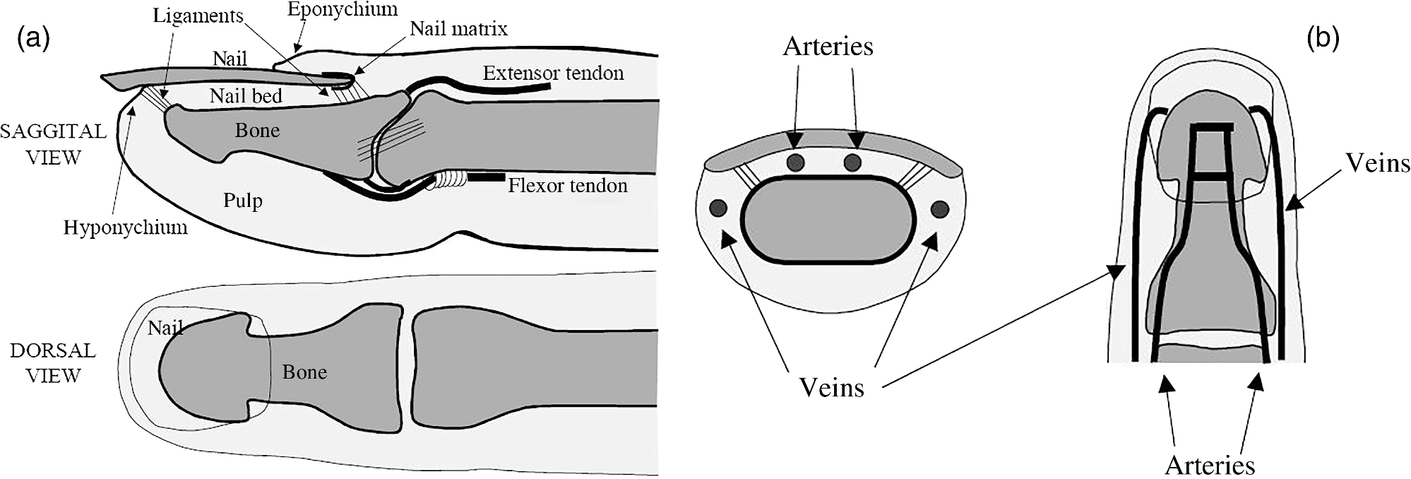
1.IntroductionPulse oximetry is an important medical monitoring technique. Clinicians depend on these instruments to provide accurate analyses of the oxygenation of the patient’s arterial blood.1,2 In spite of the wide use of pulse oximeters, the relationship between arterial oxygen saturation and their readings is not well understood.3–5 However, a major shortcoming of the current transmission oximeters is the requirement of a cuvette through which light signals must be transmitted, thus limiting its application to the fingertip or earlobe. The fingertip type pulse oximeter is commonly used in hospitals to provide basic physiological parameters. However, it is inconvenient for long-term monitoring in daily life for the frequent usage of fingertips, making the monitored signal unstable and causing variation of the oxygen saturation value. Therefore, it is important to develop other types of pulse oximeters, such as reflectance pulse oximeters. In the other words, more broad applications can be achieved with the reflectance mode. The reflectance pulse oximeter, as reported by Mendelson et al.,6 was the first to measure arterial oxygen saturation from the fingertip. Since then, several reflectance pulse oximeters have been reported.7,8 Reflectance pulse oximetry monitors arterial oxygen saturation noninvasively by measuring the intensity of red and infrared light backscattered from the skin. The technique is based on the detection of the differences in light absorption between reduced hemoglobin (Hb) and oxyhemoglobin () in a pulsating vascular bed. Skin reflectance oximetry enables the measurement of from more centrally located parts of the body, such as the forearms, chest, and forehead, which cannot be monitored by conventional transmission pulse oximetry techniques. The many factors influencing the accuracy and availability of arterial oxygen saturation measurement are difficult to investigate in vivo, especially in clinical practice. This has stimulated interest in mathematical modeling of light in tissue to gain insight into the phenomena underlying pulse oximetry. The purpose of this paper is to develop the diffusion theory to model the response of reflection pulse oximeters in multilayer biological tissues. For this purpose, we report a model for magnitude of the intensity captured by the reflected and the transmitted light detectors. This model is obtained by analyzing light propagation through tissue using the analytical solutions (AS) of the diffusion approximation equation at a given set of tissue characteristics. Analytical models based on partial differential equation (PDE) using the finite element method (FEM) and finite difference (FD) can be used to solve the diffusion equation. Furthermore, there are stochastic models, such as Monte Carlo (MC) or random-walk, to solve the above-mentioned equation. Among these models, MC has the highest accuracy in modeling, but this method requires a prohibitive amount of computational time due to the large number of photons required to obtain statistically useful data.9 Also, FD methods are not feasible for irregular boundaries because these methods use rectangular mesh elements.10,11 Since FEM offers advantages in flexibility and speed in solving complex geometries and heterogeneous tissues, researchers have preferred this method.10,12 In addition, the FEM has been used for two-dimensional and three-dimensional (3-D) geometries using linear functions by three-node triangular elements. Also, the FEM is much more efficient and accurate in comparison with the MC methods.13 At the first time, the heterogeneous tissue close to the anatomical structures of fingertip was modeled to obtain more accurate results. In addition, the light propagation was simulated accurately with our proposed model. The accuracy and reliability of data obtained with a reflection model were compared to those obtained with a transmission model. Also, the performance and accuracy between AS and FEM have been investigated by comparing the obtained results with MC simulation as a gold standard. Furthermore, it was shown that the proposed model had sufficient accuracy by comparison with data obtained from the experimental study. 2.Materials and MethodsLight propagation through scattering media has attracted great attention in many areas of physics, biology, medicine, and engineering. The radiative transfer equation,14 as a complex integrodifferential equation, is used to describe this process. Also, this equation is reduced to the diffusion equation under the strong scattering conditions, but it does not provide exact solutions in the majority of cases. 2.1.Model Structure2.1.1.Structure of the fingertipDetails of the anatomical structure of the fingertip can be found in several references.15–17 The sagittal cross section of the fingertip and skin model has been shown in the top of Fig. 1(a). The bone of the distal phalanx is surrounded beneath by the soft deformable tissue of the pulp and above by the nail unit. The nail bed is richly vascularized with blood flowing from the digital arteries into a network of arterioles, through capillary loops just under the surface, and back out through the venules to the digital veins. Figure 1(b) shows a diagram of the principal arteries and veins. The digital arteries measure is in diameter.18 There are approximately three or more arteries that take off from the distal arch measuring .18 The venous anatomy is significantly variable and consists of a dorsal and palmar system.19,20 Figure 2 presents the radiographic measurements of the distal phalanx using GE Imagecast PACS, and Table 1 shows the overall mean for measurement.21 These data were averaged and further used as the referencing data in the simulation of phantom. Table 1Mean dimension by finger.
2.1.2.Optical propertiesThe optical parameters of human skin layers are shown in Fig. 3 and Table 2.22 Evidently not all parameters for skin layers are known yet; some of them were extrapolated. Especially, for anisotropy factor , there is the lack of experimental data. Fig. 3Skin model: 1, epidermis; 2, dermis; 3, dermis with plexus superficialis; 4, dermis; 5, dermis with plexus profundus; and 6, subcutaneous tissue.  Table 2Optical properties of the different layers of the tissue model.
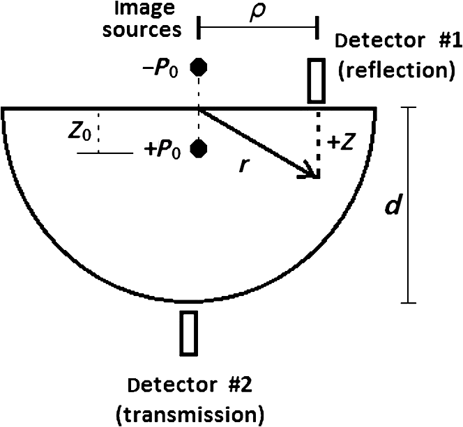
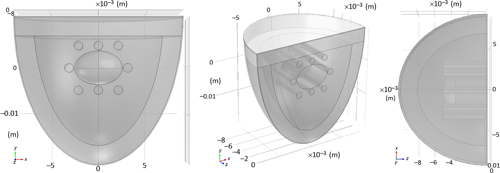
2.1.3.Geometry of modelIn this paper, a hemispherical volume of tissue is used to represent the tip of a finger on which an oximeter probe is placed. The geometry of the problem is illustrated in Fig. 4. The light source is modeled as a point source emitting monochromatic light at a wavelength in the near-infrared (NIR) region of the spectrum. For mathematical convenience, the point source is represented as a dipole composed of a photon source and a photon sink. The detector receives light at a point opposite to the source (transmission case) or at a point on the same side as the source (reflection case). The finger is treated as a heterogeneous mixture of blood and other tissues containing no blood, and its optical properties are assumed to be determined mostly by dermal and subcutaneous tissues. The pigmented epidermis, which is very thin () and scatters light mostly in the forward direction,23 is neglected in this analysis because it only serves to attenuate the source light before and after it undergoes absorption and scattering in the blood-perfused tissue. 3.Theory3.1.Detection Light IntensityGenerally, the detected light intensity of a reflection pulse oximeter is weaker than that of a transmission pulse oximeter with the same source–detector separation. To determine the detectable light intensity of a pulse oximeter, we calculated the detected light for reflection and transmission modes using the analysis of light propagation in tissue. 3.1.1.Diffusion approximation implementation in numerical methodsPartial differential equation representation of diffusion approximationThe theory of diffusion approximation is based on the radiative transport equation and the conservation of energy. This equation is in general not amenable to an analytic solution for arbitrary light input. Only in specific and restricted geometries are closed-form solutions known.24,25 The radiative transport equation in a media that scatters and absorbs photons is where is the average power flux density at point in the direction of unit vector , at time , in the unit of (). is the speed of light in the medium. is the optical transport coefficient, where is the scattering coefficient and is the absorption coefficient. is the spatial and angular distribution of the source in the unit of (). The normalized phase function represents the probability of scattering in a direction from direction .Various tissue optical properties, such as the absorption coefficient, scattering coefficient, anisotropy index, and refractive index, can be used to calculate the power distributions and trajectories of photons. The scattering behavior is usually described by the Henyey–Greenstein phase function.26 The photons pass that through and interact with scatterers in the biological tissue are subject to a high degree of forward scattering. The phase function describes the power distribution of scattering from the forward direction (0 deg) to the backward direction (180 deg), and its equation is given by where denotes the scattered intensity at a specific angle and and denote a normalization parameter and the direction of scattering, respectively. Parameter , named the scattering anisotropy parameter, denotes the mean cosine of the scattering angle and is given byWe use Eq. (2) to obtain the normalized scattering phase function. Figure 5 shows the phase-function diagrams at 656 and 943 nm for different tissues: epidermis, dermis and pulp, bone, and blood. Since scattering anisotropy parameter is close to 1, the diagrams exhibit a sharp peak at 0 deg, which indicates that light tends to scatter in the forward direction during interactions between photons and biological tissues. Fig. 5Normalized angular scattering intensity distributions for epidermis, dermis and pulp, bone, and blood at (a) 656 and (b) 943 nm.  On the other hand, treating the tissue as a heterogeneous mixture, the total absorption coefficient can be written as a sum of the absorption coefficients of the individual tissue components where and are the volume fractions of arterial and venous blood, respectively, and is the absorption coefficient of the bloodless tissue. The absorption coefficients of the arterial and venous blood in the above equation are and , respectively.Like the absorption coefficient, the total scattering coefficient of the idealized heterogeneous tissue can also be written as a sum of the coefficients of the individual tissue components where and are the scattering coefficients of whole blood and of the component of the tissue containing no blood, respectively.The photon fluence is given by The photon flux or current density is given by Both the fluence and the flux are in units of . In vivo experimental light propagates in a highly scattering tissue in which the scattering coefficient is considerably greater than the absorption coefficient and the diffusion approximation is sufficiently accurate. In the approximation, the radiance is expanded in spherical harmonics truncated to the first order, and the radiance equation can be reduced to the time-dependent diffusion equation 27,28 where is the photon fluence rate and is the diffusion coefficient.The steady-state diffusion equation for the average diffuse intensity in a heterogeneous scattering medium of absorption coefficient is Analytical solution of PDE representation of diffusion approximation:With dimensional parameters defined in Fig. 4, the diffusion approximation equation, by considering the approximation of in a highly scattering tissue, is as follows: where is the reduced scattering coefficient and is the effective attenuation coefficient. An explanation of these coefficients in the context of diffusion theory as applied to biological tissues can be found in a review by Cheong et al.29 For a point source, can be written in terms of the volume delta function , as below: where is the power emitted by the source. We will first solve Eq. (10) for within a bounded spherical medium and then derive the solution for the hemispherical geometry as depicted in Fig. 4 from this result using the method of images.30The general solution to Eq. (10) is where and are the constants determined by two boundary conditions. The first boundary condition is as follows: where denotes the flux of fluence rate.The second boundary condition is that all photon flux is absorbed beyond the boundary Subsequently, is, for bounded spherical geometryAlso, the AS of the diffusion approximation equation for a point beam incident on the surface of a semi-infinite medium is given by summing the solutions for a pair of positive and negative point sources as follows: where is the depth from the surface and is the distance between the point of interest and the -axis, as shown in Fig. 4. and are given as follows: In these equations, is the distance between the real and extrapolated boundaries for the refractive index mismatched case. is a small value representing the depth below the surface from which the first-scattered photons emanate. We assume here that the incident photons are converted to scattered photons within one mean scattering length, so is simply given as where is related to the internal reflection and can be derived from Fresnel reflection coefficients.31 When the boundary has matched refractive indices, ; otherwise, is estimated as32 where where is the relative index of tissue to air. Now, by applying the method to images, the desired solution for hemispherical geometry can be obtained from Eq. (16)The magnitude of the intensity captured by the reflected light detector (labeled “#1” in Fig. 4) is given by The magnitude of the intensity captured by the transmitted light detector (labeled “#2” in Fig. 4) is given by From the above equations, a model of the response from a pulse oximeter can be developed.Numerical method to solve the diffusion approximation equationFinite element method:In this section, the FEM model has been used to perform the forward problem of light propagation in scattering tissue. Numerical experiments:Due to the accuracy and efficiency of FEM, we used this method to calculate solutions of the diffusion approximation equation along with the Dirichlet boundary conditions (DBC) and Robin boundary conditions (RBC) presented in Eqs. (26) and (27), respectively,33 where is the normal vector.Assumptions used in the FEM formulation is that is continuous and approximately obeys the diffusion equation locally within the domain . To find a piecewise linear approximation and continuous function of , is divided into nonoverlapping elements , such that , joined at vertex nodes. Then, the solution obtained for is approximated by a piecewise polynomial and continuous function as where the set is the basis function set for expansion. Considering these assumptions, the diffusion Eq. (8) is declared as12,18 where where is the basis function and is the test function.By considering the time-independent case, the equation can be written as Following the above derivation, the equation was obtained as where , , , , and have the same meaning as mentioned earlier.The above explanation of the FEM discretization preserves the frequency-domain differential equation (DE). Also, associating the Robin boundary condition, which can be expressed as where is considered as 0.177 for a tissue–air interface and is the unit vector normal to the boundary, the DE discrete formulation in the frequency domain can be explained as where and exhibit the source values and nodal solution, respectively, , , and are system matrices as described above, and .Optical simulation model of fingertip:The finger base mainly consists of epidermis, phalanx, blood, and dermis and pulp. The fingertip model used in this work has been illustrated in Fig. 6. In this model, the height, thickness, and outer epidermis’ thickness of employed geometry are 15, 10, and 0.1 mm, respectively. Also, the characteristics of distal phalanx have been listed in Table 1. As defined in Sec. 2.1.1, three pairs of arteries with 0.85-mm diameter are considered top and bottom of the distal phalanx. Additionally, there are several veins with 0.85-mm diameter on both sides of the distal phalanx. Table 3 shows the different tissues optical properties at wavelengths 656 and 943 nm.9–35 In the simulated model, the wavelength of 943 nm and a fixed intensity have been employed for the light point source. Table 3Optical properties used in the tissue simulations: μa (absorption coefficient), μs (scattering coefficient), n (refractive index), and g.
Mesh generation:In this study, the developed model involved hemispherical geometry and heterogeneous cases. To improve the accuracy of the geometry approximation, six node triangular elements were used instead of three nodes. Also, more accurate answers were obtained by using a quadratic shape function in comparison of three-node linear triangular elements. Figure 7 illustrates the six node triangular elements in the model. 3.1.2.Monte Carlo simulationAs a gold standard, MC simulation was used to validate the effectiveness of FEM and AS in this research. The transport of photons was tracked. The anisotropy factor and the refractive index of the tissue were assumed in accordance with Table 3. The medium above and beneath the tissue was treated as air, with a refractive index of 1.0. Thus, the boundary between the tissue and air was mismatched. The specular reflection would occur after photons had been launched. The Henyey–Greenstein phase function expressed by Eq. (2) was used to describe photon scattering. The spatial resolution for both radial and depth distance was set at 0.01 mm, which is more than enough for real applications. After sufficient propagation in the tissue, the photon packets would be terminated by reflection or transmission out of the tissue. The weights of the photon packets that exited the tissue were accordingly scored into the diffuse reflectance or diffuse transmittance, depending on where the photon packets exited.36 To obtain diffuse reflectance caused by the finite size beam, the light beam of finite size was assumed to be collimated, and the response was computed from the convolution of the response of an infinitely small beam, according to the profile of the finite size beam.37,38 A publicly available MC code (MCML) for light propagation in biological materials provided by Wang et al.36 was used. 3.1.3.Experimental studyThe purpose of experiments is to validate and evaluate the performance of the mathematical model by making measurements of steady-state intensity over the tissue geometry. Experiments on 19 healthy volunteers were conducted. All of the volunteers who participated in the study were males with ages ranging between 18 to 43 years with the mean and standard deviation of 27.36 and 7.55, respectively (see Table 4). This study was approved by the ethics committee of the Shahid Beheshti University of Medical Sciences. Table 4Biometric detail of the volunteers that was investigated in the study.
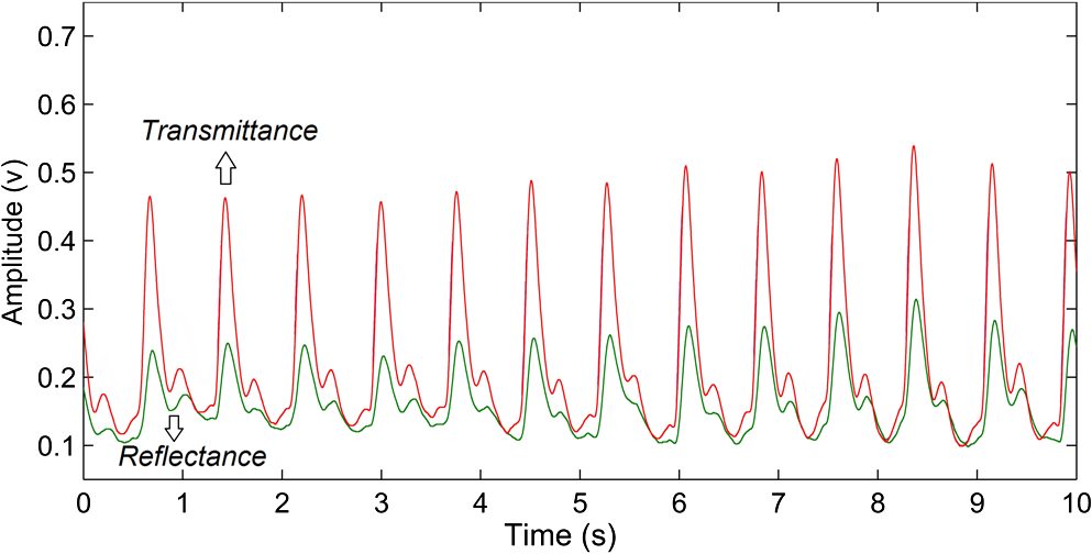
In pulse oximeters, the arterial oxygen saturation is calculated as a function of the ac/dc ratio of detected light intensity at systole and diastole. Here, the change of the blood volume due to the heart diastole and heart systole leads to the varying signal of light absorption that is called a photoplethysmograph (PPG). The pulse oximeter can calibrate and estimate by the parameter of ratio obtained from the PPG signal. The defining equation is where where and denote the DC and AC components of the PPG signal for red light, respectively. and denote the DC and AC components of the PPG signal for NIR light, respectively. The function is determined by the manufacturer from clinical and in vitro studies.A PPG finger probe that operates in transmittance and reflectance mode has been used. Eight PPG signals were recorded from the reflectance and transmittance PPG system, consisting of four PPG signals (red DC and AC and infrared DC and AC signals) acquired from each mode that represents values. Figures 8 and 9 show a sample of the two infrared and red AC PPG signals, respectively, obtained from the transmittance and reflectance PPG systems of one volunteer. 4.Results and DiscussionIn this section, the FEM model and AS presented in the previous sections were evaluated. We have implemented the FEM and MC methods, which incorporate the boundary and source conditions discussed above. The obtained outcomes compared against MC simulations as a gold standard. Furthermore, experimental data were used for the evaluation and comparison of the models obtained for light intensity of reflection and transmission pulse oximeters. 4.1.Simulation Results of Finite Element MethodA point source is present just inside the boundary of the tissue. The radial location of the source was positioned inside the physical boundary by a distance, for the point source excitation used in the computational algorithm.39–41 It is worth mentioning that, the resolution of the mesh plays an important role for the stability and accuracy of the FEM model. Meshing is done to divide the entire specimen into nodes where the partial differential equation can be solved. The mesh is intensified where the source is present as it is the area of interest. The mesh of our structure is presented in Fig. 10, we use free mesh parameters with a maximum element size scaling factor = 1, a maximum element growth rate = 1.5, a mesh curvature factor = 0.6, a mesh curvature cutoff = 0.001, and a resolution of narrow region = 0.5. Figure 11 depicts the propagation of light waves around the point source by the contours. Contours are close together in the proximity of the light source and further toward the other side. Point source has a fixed intensity. Fluence values are found throughout the specimen. The values of absorption and reduced scattering coefficients inside the specimen are known (see Fig. 12). Figure 13 illustrates the simulated flux density by considering the optimal boundaries. Also, a continuous flux can be seen between the two layers and when moving outward from the two media. Figure 14 shows the cross section through the photon density distribution along the -, -, and -axes for the FEM model, on a logarithmic scale. In all three cases, the equivalent isotropic source is placed at position . 4.2.Comparison Between Reflectance and Transmittance Modes and Investigation with Experimental DataA reflectance oximeter has sensing and emitting diodes on a single surface. Therefore, they can be placed in an anatomical location that does not require two surfaces in close proximity. In addition, their advantage is that, regardless of the patient’s age or size (infants to very large adults), it provides more accurate and stable readings. The light is emitted by the LEDs, passes through blood vessels and tissue, then reflects off the bone, and passes through the tissues once more, where a significant amount of light will reflect off the skin in the reflectance setup. Thus, reflectance probes have a lower signal-to-noise ratio and a higher offset than the transmittance probes. Also, reflectance setups require a significantly greater amount of light because the detected light intensity of a reflection pulse oximeter is weaker than that of a transmission pulse oximeter with the same source–detector separation (see Fig. 15). Fig. 15At the same source–detector separation: (a) light intensity of the reflection pulse oximeter obtained from FEM simulation and (b) light intensity of the transmission pulse oximeter obtained from FEM simulation.  The simulation results and measurement (experimental data) are compared. Figure 16 shows the results of the measurements and corresponding simulations. They show an overall good agreement. As can be seen, the ratio between measured and simulated values is almost constant; hence, the characteristics of the light propagation can be accurately reproduced. 4.3.Comparison of Monte Carlo, the Analytical Method, and Finite Element MethodIn this section, diffuse reflectance AS for fingertip geometry given by Eq. (24) is validated using the MC method. The optical parameters used are presented in Table 3 and under optical simulation model of fingertip. Also, the fluence rates generated by MC, the analytical method, and FEM were compared at a radial distance . First, all generated profiles were normalized at a depth of 5 mm; then, they were normalized at a distance of 2 mm, which is out of the region of 1 mean free path (mfp) from the isotropic point source. A reduced scattering albedo (RSA) defined by was used to measure the ratio of photon scatting to absorption. The relative refractive index of the boundary was set at 1.37. Figures 17Fig. 18–19 present a comparison between the FEM and AS for RSAs 45.82, 35.05, and 10.56, respectively. As a result, the relative errors between the photon fluence rate obtained from the FEM model and from the AS were 8.9%, 6.4%, and 3.8% for RSAs of 45.82, 35.05, and 10.56, respectively. Figures 20 and 21 show for matched and mismatched boundary conditions that AS and MC results do not exactly match near the sources. Furthermore, by comparison of both type of boundary conditions, it can be observed that solutions begin to match after some reduced mfp, that is nearer to the source in case of matched. Fig. 20Comparison of AS of diffuse reflectance with the MC method for (a) matched boundary and (b) relative error.  Fig. 21Comparison of AS of diffuse reflectance with the MC method for (a) mismatched boundary and (b) relative error.  Figures 22 and 23 show the fluence rate profiles and relative errors on a logarithmic scale. Except for a small depth region within 1 mfp of the surface, FEM simulated the distribution of internal fluence rate accurately, compared to MC simulation, with relative errors of less than 3%. For the small depth region close to the light source, FEM simulated the distribution of internal fluence with relative errors of less than 9%, compared to MC simulation. These findings also agree with that of Schweiger et al.42 Fig. 22(a) Fluence rate along the axis in the tissue simulated by MC and FEM and (b) relative errors with respect to MC simulation. 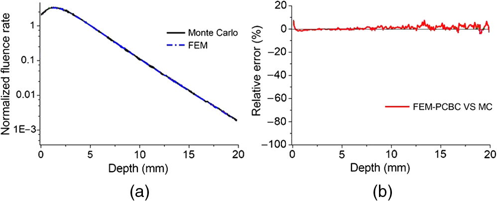 Fig. 23(a) Fluence rate obtained using MC, the analytical method, and FEM and (b) their relative errors, compared to MC simulation.  According to the simulation results shown in Fig. 23, all methods underestimated the fluence rate at the boundary by a large error within the region of 1 mfp close to the light source because diffusion approximation was not valid in this region. Furthermore, the analytical method and FEM performed about the same over the entire distances. It can thus be concluded that, overall, the analytical method and FEM have almost identical results compared with MC as the gold standard. The differences are so small between FEM and AS that it is possible to use the diffusion theory for the analysis and prediction of the response of pulse oximeters. Also, it is obvious that the FEM is much more efficient and accurate than the AS method in heterogeneous advanced tissue and has the ability to estimate fluence distribution in highly complex geometries, thus making it a very useful tool in quantifying the optical parameters. 4.4.Comparison Experimental Results with Finite Element Method and Analytical SolutionDiffuse reflectance defines mainly the light coming out from the medium and diffusely entered into the medium from outside. It depends strongly on the tissue optical properties and is mainly required to determine the optical properties of the medium. Here, a comparative study has been done for diffuse reflectance calculated using FEM and AS for fingertip geometry with respect to different scattering and absorption coefficients. Later, conclusions are presented based on this study. The purpose of experiments is to validate the analytical and FEM models by making measurements of steady-state intensity over the fingertip geometry. Pulse oximeters use the red and infrared maximum and minimum detected light intensities to calculate . In this study, our model works in reverse. To obtain experimental data for light intensities, the is input and the resulting transmitted and reflected light intensities are calculated to compare with diffuse reflectance values calculated using 3-D FEM and AS. The FEM solution is almost matching with the experiment result. AS is coming as per our expectations, as it has been analyzed that AS is approximately matching with FEM solution (see Fig. 24). Also, Fig. 24 shows good agreement between the numerical results and the experimental results. This study helps us to reach a conclusion for the feasibility of the diffusion approximation equation for the investigation of reflectance pulse oximeter in NIR region. 5.ConclusionsWe have developed a theoretical model for photon migration through scattering media in the presence of an absorbing inhomogeneity. A 3-D model of a phantom, which had similar properties to that of a human fingertip tissue, was simulated. Furthermore, the FEM was applied to the diffusion approximation equation for modeling light propagation in the fingertip. These models have been verified by MC simulation and experimental data for use in biomedical optical imaging studies. The results of the presented models have a good match with MC simulation and experimental data. To the best of our knowledge, no published model provides a good match to experimental data. This research shows that it is possible to model a reflectance pulse oximetry with diffusion theory. The aim of this paper was to demonstrate the power of the FEM and AS in modeling the steady-state diffusion equation in a heterogeneous medium. The FEM now allows us to select the model that matches a given experimental situation best. Also, since FEM is fast and capable of dealing with complex geometries and different beam profiles, it is advantageous to use the method. To find the conditions that correspond between real experiments and FEM, more work will be required. In particular, the source model requires more attention; neither the simple isotropic source at a depth of nor the diffuse boundary current is appropriate. The correct model may have to take into account angular weighing, spatial distribution, and other factors. However, the major benefit of the model is in estimating the effects of various physical and physiological variables on pulse oximeters. Also, the model presented in this paper helps to explicitly delineate the roles of absorption and scattering in diffuse reflectance. The results from both FEM and AS validate that the diffusion approximation equation could resolve the heterogeneous advanced tissue. In addition, the results show that FEM could offer the simulation with higher efficiency and accuracy. DisclosuresProfessor Setayeshi has nothing to disclose. Dr. Mehrabi has nothing to disclose. Dr. Ardehali has nothing to disclose. Dr. Arabalibeik has nothing to disclose. No conflicts of interest, financial or otherwise, are declared by the authors. ReferencesK. J. Reynolds et al.,
“In vitro performance test system for pulse oximeters,”
Med. Biol. Eng. Comput., 30
(6), 629
–635
(1992). http://dx.doi.org/10.1007/BF02446795 MBECDY 0140-0118 Google Scholar
M. Cannesson et al.,
“Respiratory variations in pulse oximetry plethysmographic waveform amplitude to predict fluid responsiveness in the operating room,”
J. Am. Soc. Anesthesiol., 106
(6), 1105
–1111
(2007). http://dx.doi.org/10.1097/01.anes.0000267593.72744.20 Google Scholar
M. Elliott et al.,
“Do clinicians know how to use pulse oximetry? A literature review and clinical implications,”
Aust. Crit. Care, 19
(4), 139
–144
(2006). http://dx.doi.org/10.1016/S1036-7314(06)80027-5 Google Scholar
S. Fouzas et al.,
“Knowledge on pulse oximetry among pediatric health care professionals: a multicenter survey,”
Pediatrics, 126
(3), e657
–e662
(2010). http://dx.doi.org/10.1542/peds.2010-0849 PEDIAU 0031-4005 Google Scholar
D. R. Marble et al.,
“Diffusion-based model of pulse oximetry: in vitro and in vivo comparisons,”
Appl. Opt., 33
(7), 1279
–1285
(1994). http://dx.doi.org/10.1364/AO.33.001279 APOPAI 0003-6935 Google Scholar
Y. Mendelson et al.,
“Spectrophotometric investigation of pulsatile blood flow for transcutaneous reflectance oximetry,”
Oxygen Transport to Tissue-IV, 93
–102 1st ed.Plenum Press, Springer, New York
(1983). Google Scholar
Y. Mendelson et al.,
“Design and evaluation of a new reflectance pulse oximeter sensor,”
Med. Instrum., 22
(4), 167
–173
(1988). MLISBY 0090-6689 Google Scholar
Y. Mendelson and B. D. Ochs,
“Noninvasive pulse oximetry utilizing skin reflectance photoplethysmography,”
IEEE Trans. Biomed. Eng., 35
(10), 798
–805
(1988). http://dx.doi.org/10.1109/10.7286 IEBEAX 0018-9294 Google Scholar
O. Zhernovaya et al.,
“The refractive index of human hemoglobin in the visible range,”
Phys. Med. Biol., 56
(13), 4013
–4021
(2011). http://dx.doi.org/10.1088/0031-9155/56/13/017 PHMBA7 0031-9155 Google Scholar
S. R. Arridge and J. C. Hebden,
“Optical Imaging in medicine II: modeling and reconstruction,”
Phys. Med. Biol., 42
(5), 841
–853
(1997). http://dx.doi.org/10.1088/0031-9155/42/5/008 PHMBA7 0031-9155 Google Scholar
A. J. Welch et al.,
“Definitions and overview of tissue optics,”
Optical Thermal Response of Laser Irradiated Tissue, 15
–46 1st ed.Plenum, Springer, New York
(1995). Google Scholar
M. Schweiger et al.,
“The finite element method for the propagation of light in scattering media: boundary and source conditions,”
Med. Phys., 22
(11), 1779
–1792
(1995). http://dx.doi.org/10.1118/1.597634 MPHYA6 0094-2405 Google Scholar
Y. Xu and Q. Zhu,
“Comparison of finite element and Monte Carlo simulations for inhomogeneous advanced breast cancer imaging,”
in Excerpt from the Proc. of the COMSOL Conf. Boston,
(2010). Google Scholar
K. M. Case and P. F. Zweifel, Linear Transport Theory, Addison-Wesley Publishing Co., Reading, Massachusetts
(1967). Google Scholar
R. K. Scher and C. R. Daniel, Nails: Therapy-Diagnosis-Surgery, 2nd ed.W.B. Saunders, Philadelphia
(1990). Google Scholar
P. Valentine, R. Tubiana,
“Physiology of extension of the fingers,”
The Hand, 1 WB Saunders, Philadelphia
(1981). Google Scholar
R. Baran et al., Diseases of the Nails and their Management, 2nd ed.Blackwell Scientific, Oxford
(1994). Google Scholar
D. O. Smith et al.,
“Artery anatomy and tortuosity in the distal finger,”
J. Hand Surg., 16
(2), 297
–302
(1991). http://dx.doi.org/10.1016/S0363-5023(10)80114-5 JHSUDV 0266-7681 Google Scholar
D. O. Smith et al.,
“The distal venous anatomy of the finger,”
J. Hand Surg., 16
(2), 303
–307
(1991). http://dx.doi.org/10.1016/S0363-5023(10)80115-7 JHSUDV 0266-7681 Google Scholar
G. L. Lucas,
“The pattern of venous drainage of the digits,”
J. Hand Surg., 9
(3), 448
–450
(1984). http://dx.doi.org/10.1016/S0363-5023(84)80242-7 JHSUDV 0266-7681 Google Scholar
M. Darowish et al.,
“Dimensional analysis of the distal phalanx with consideration of distal interphalangeal joint arthrodesis using a headless compression screw,”
Hand, 10
(1), 100
–104
(2015). http://dx.doi.org/10.1007/s11552-014-9679-x Google Scholar
V. V. Tuchin and V. Tuchin, Tissue Optics: Light Scattering Methods and Instruments for Medical Diagnosis, 2nd ed.SPIE Press, Bellingham, Washington
(2007). Google Scholar
W. A. Bruls and J. C. Van Der Leun,
“Forward scattering properties of human epidermal layers,”
Photochem. Photobiol., 40
(2), 231
–242
(1984). http://dx.doi.org/10.1111/j.1751-1097.1984.tb04581.x PHCBAP 0031-8655 Google Scholar
A. Ishimaru, Wave Propagation and Scattering in Random Media, Academic Press, New York
(1978). Google Scholar
K. Shimizu,
“Remote sensing of microparticles by laser scattering for medical applications,”
University of Washington,
(1979). Google Scholar
V. V. Tuchin,
“Light scattering study of tissues,”
Phys. Usp., 40
(5), 495
–515
(1997). http://dx.doi.org/10.1070/PU1997v040n05ABEH000236 PHUSEY 1063-7869 Google Scholar
D. A. Boas,
“Diffuse photon probes of structural and dynamical properties of turbid media,”
University of Pennsylvania,
(1996). Google Scholar
S. R. Arridge et al.,
“A finite element approach for modeling photon transport in tissue,”
Med. Phys., 20
(2), 299
–309
(1993). http://dx.doi.org/10.1118/1.597069 MPHYA6 0094-2405 Google Scholar
W. F. Cheong et al.,
“A review of the optical properties of biological tissues,”
IEEE J. Quantum Electron., 26
(12), 2166
–2185
(1990). http://dx.doi.org/10.1109/3.64354 IEJQA7 0018-9197 Google Scholar
R. J. Fretterd and R. L. Longini,
“Diffusion dipole source,”
J. Opt. Soc. Am., 63
(3), 336
–337
(1973). http://dx.doi.org/10.1364/JOSA.63.000336 Google Scholar
J. G. Webster, Design of Pulse Oximeters, CRC Press, Bristol
(1997). Google Scholar
R. A. Groenhuis et al.,
“Scattering and absorption of turbid materials determined from reflection measurements. 1: theory,”
Appl. Opt., 22
(16), 2456
–2462
(1983). http://dx.doi.org/10.1364/AO.22.002456 APOPAI 0003-6935 Google Scholar
S. Abdelali and M. Karim,
“Resolution of direct problem by the finite element method: application in near infra-red optical medical imaging,”
Dig. J. Nanomater. Biostructures, 7
(3), 1271
–1277
(2012). Google Scholar
D. J. Faber et al.,
“Oxygen saturation-dependent absorption and scattering of blood,”
Phys. Rev. Lett., 93
(2), 028102
(2004). http://dx.doi.org/10.1103/PhysRevLett.93.028102 PRLTAO 0031-9007 Google Scholar
H. Ding et al.,
“Refractive indices of human skin tissues at eight wavelengths and estimated dispersion relations between 300 and 1600 nm,”
Phys. Med. Biol., 51
(6), 1479
–1489
(2006). http://dx.doi.org/10.1088/0031-9155/51/6/008 PHMBA7 0031-9155 Google Scholar
L. Wang et al.,
“MCML-Monte Carlo modeling of light transport in multi-layered tissues,”
Comput. Methods Programs Biomed., 47
(2), 131
–146
(1995). http://dx.doi.org/10.1016/0169-2607(95)01640-F CMPBEK 0169-2607 Google Scholar
S. A. Prahl et al.,
“A Monte Carlo model of light propagation in tissue,”
Dosim. Laser Radiat. Med. Biol., 5 102
–111
(1989). Google Scholar
L. Wang and S. L. Jacques, Monte Carlo Modeling of Light Transport in Multi-Layered Tissues in Standard C, University of Texas MD Anderson Cancer Center, Houston
(1992). Google Scholar
K. D. Paulsen and H. Jiang,
“Spatially-varying optical property reconstruction using a finite element diffusion equation approximation,”
Med. Phys., 22
(6), 691
–701
(1995). http://dx.doi.org/10.1118/1.597488 MPHYA6 0094-2405 Google Scholar
H. Jiang et al.,
“Optical image reconstruction using frequency-domain data: simulations and experiments,”
J. Opt. Soc. Am. A, 13
(2), 253
–266
(1996). http://dx.doi.org/10.1364/JOSAA.13.000253 JOAOD6 0740-3232 Google Scholar
S. R. Arridge et al.,
“A finite element approach for modeling photon transport in tissue,”
Med. Phys., 20
(2), 299
–309
(1993). http://dx.doi.org/10.1118/1.597069 MPHYA6 0094-2405 Google Scholar
M. Schweiger et al.,
“The finite element method for the propagation of light in scattering media: boundary and source conditions,”
Med. Phys., 22
(11), 1779
–1792
(1995). http://dx.doi.org/10.1118/1.597634 MPHYA6 0094-2405 Google Scholar
BiographyMohsen Mehrabi is currently a PhD student at Amirkabir University of Technology of Iran, under the tutelage of Professor Saeed Setayeshi. He earned his master’s degree at Amirkabir University of Technology in 2011. His research focuses on biomedical instruments, optical electronics, and medical processing. Saeed Setayeshi, MA, MSc, MASc, PhD, PEng, received his PhD in electrical engineering in Canada in 1993. His research interests are in the areas of intelligent control (neural–fuzzy–expert), adaptive signal processing, medical imaging, optical electronics, LCD design, and knowledge-based systems. Currently, he is an associate professor at the Department of Energy Engineering and Physics, Amirkabir University of Technology, Tehran, Iran. Seyed Hossein Ardehali received his MD degree from Islamic Azad University in 1995, his national board certificate from Iran University of Medical Sciences in 2001, and a fellowship of critical care medicine from Shahid Beheshti University of Medical Sciences in 2006. Now, he is the director of the intensive care ward at the Shohadaye Tajrish Hospital, Shahid Beheshti University of Medical Sciences. He has contributed to more than 15 articles about critical care medicine. Also, he is member of the board of the Iranian Critical Care Society. Hossein Arabalibeik received his BSc and MSc degrees in electrical engineering from Iran University of Science and Technology. He obtained his PhD in nuclear engineering from Amirkabir University of Technology, Tehran, Iran, in 2003. In 2005, he joined Tehran University of Medical Sciences, where he works on developing laser systems for skin treatment and medical instruments. |