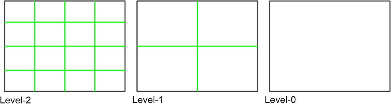
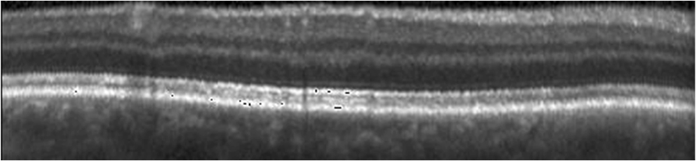
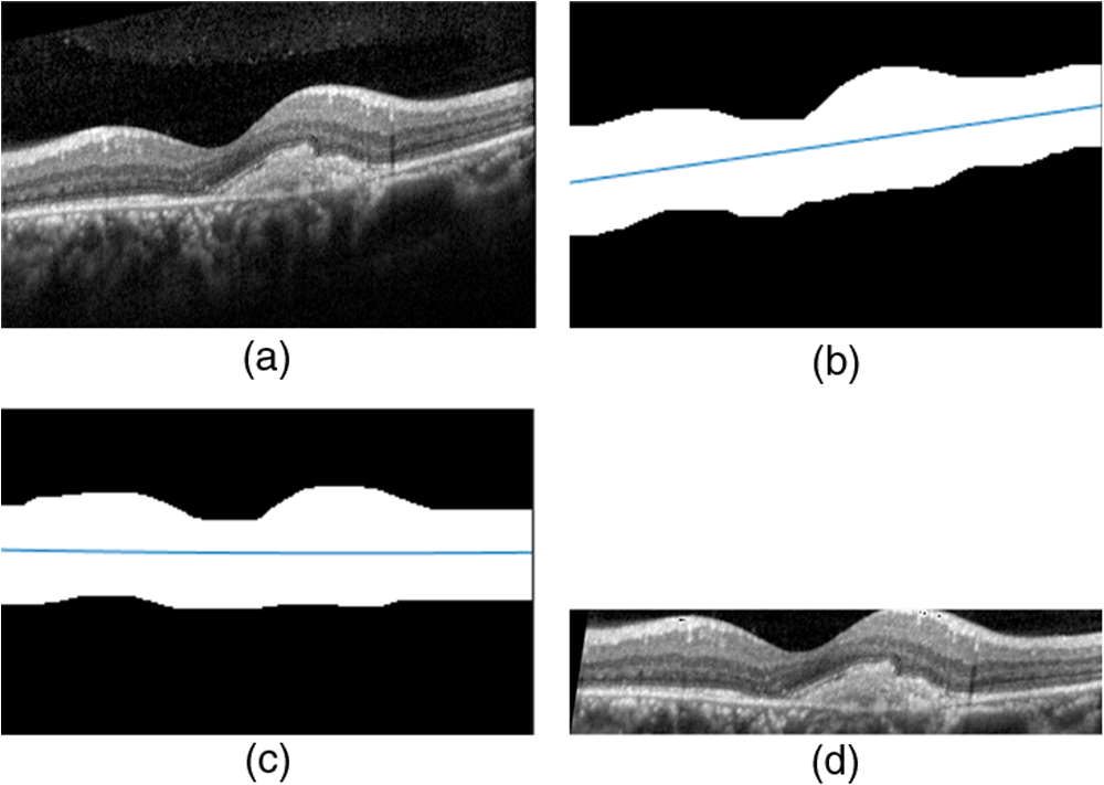
2.1.

Image Preprocessing

OCT images are usually rife with speckles and the position of the retina varies substantially among scans, which makes it nontrivial to align all the retina areas into a relatively unified position. Therefore, an aligning method for preprocessing is necessary. However, considering the previous works, there are three issues that we have taken into consideration. First, Srinivasan et al.²⁷ aligned retina regions by fitting a second-order polynomial to the RPE layer and then flattened the retina. However, their method is invalidated once the RPE layer of the retina is too severely distorted to fit the curve of the RPE boundary of the retina [as depicted in Fig. 1(b)]. Second, Liu et al.²⁴ aligned retina regions by fitting a second-order polynomial to the whole retina OCT image. Although their aligning method could deal with retina images that contain distorted RPE layers, the effectiveness of their method is seriously reduced when their algorithm is employed on a certain type of diseased retina where the lesion portion is swelling up as shown in Fig. 2. Third, there are many OCT images in our datasets where the RPE layer of the retina is straight but at a certain angle with the horizontal line as shown in Fig. 5. In that case, fitting the retina with a straight line might be better than with a parabola. To solve the three problems listed above and align retinas in a more robust way, we propose a fully automated aligning method possessing three salient characteristics. First, it perceives retinas without estimating their RPE boundary. Second, it extracts two sets of data points from a given image (for linear and curved fittings) and then automatically chooses one set of data points that is more representative of the retina morphology (in our paper, the two most common morphologies of retina are considered: curved and linear). Third, it automatically decides between a second-order polynomial and a straight line to fit the set of data points being chosen. Our aligning process is illustrated in Fig. 6, taking the most common case as an example (using one of the two sets of data points and the second-order polynomial fitting). Furthermore, in Sec. 3.1, we will present and discuss more cases that previous works^24,27 have not taken into account.

Fig. 5

OCT image of a straight-strip shaped retina.

Fig. 6

Description of the image aligning process: (a) original image, (b) BM3D denoising, (c) binarizing, (d) median filtering, (e) morphological closing, (f) morphological opening, (g) polynomial fitting, and (h) retina aligning.

We separate our aligning method into three stages: perceiving stage, fitting stage, and normalizing stage.

In the perceiving stage, our method detects the overall morphology of a retina in the following steps. First, the sparsity-based block matching and 3-D-filtering (BM3D) denoising method³⁶ are used to reduce noises of the original image [Fig. 6(a)]. Second, the denoised image [Fig. 6(b)] is filtered by a threshold value to perceive the structure of the retina [Fig. 6(c)]. Third, a median filter is applied to remove detached black dots inside the retina [Fig. 6(d)], especially dots near the upper and lower edges of the white areas in Fig. 6(c), which could hamper the aligning effect in the following steps. Fourth, the morphological closing method is used to remove large black blobs inside the retina, which cannot be removed completely by the median filter [Fig. 6(e)]. Fifth, the morphological opening method is used to remove the detached white dots (caused by large noise speckles existing in some OCT scans, which are not presented in Fig. 6) outside the retina [Fig. 6(f)].

In the fitting stage, our method automatically chooses the set of data points and a fitting method, and the whole process for decision making in this stage is illustrated in Fig. 7. It could be described in two steps:

Fig. 7

Complete process of making decision on the data points and the fitting methods.

Step 1: Choosing the set of data points for fitting.

Our method extracts two sets of data points from Fig. 6(f): middle data points [i.e., each point is chosen from a unique column in the white area in Fig. 6(f), whose $x$-coordinate is the index of the column and $y$-coordinate is the arithmetic mean of $y$-coordinates of all points in the column] and bottom data points [i.e., each point is chosen from a unique column in the white area in Fig. 6(f), whose $x$-coordinate is the index of the column and $y$-coordinate is the $y$-coordinate of the corresponding bottom point in the column]. When choosing the sets of data points (the middle data points versus the bottom data points), our method performs the second-order polynomial fitting to the middle data points for judging, if the fitted parabola opens upward [Fig. 6(g)], then the middle data points are chosen; if the parabola opens downward, then the bottom data points are chosen.

Step 2: Choosing the fitting method (linear fitting versus second-order polynomial fitting).

In the case when the middle data points are chosen, our method performs the linear fitting to the data points and then calculates the correlation coefficients (calculated by using the MATLAB^® command corrcoef) between the middle data points and the two sets of the fitted points (i.e., one is from the linear fitting and another is from the second-order polynomial fitting); then the fitting method corresponding to a larger correlation coefficient is chosen [i.e., a parabola is finally chosen to fit the middle data points in Fig. 6(g) because there is a larger correlation coefficient between the middle data points and the data points to the fitted parabola (as opposed to the fitted linear line)]. In the case when the bottom data points are chosen, our algorithm performs the second-order polynomial fitting to the bottom data points for judging, if the fitted parabola opens upward, then the linear fitting is done and the fitting method with a larger correlation coefficient is chosen; if the parabola opens downward, then the linear fitting method is chosen directly.

In the normalizing stage, our method normalizes the retinas by aligning them to a relatively unified morphology and crops the images to trim out insignificant space. When the second-order polynomial fitting is chosen, the retina is flattened by moving each column of the image a certain distance according to the fitted curve [Fig. 6(h)]. In the case of the linear fitting, the retina is aligned by rotating the entire retina to an approximately horizontal position according to the angle between the fitted line and the horizontal line. When cropping the image, our method first detects the highest and lowest points of the white area when the retina region is flattened as shown in Fig. 6(h), and then, according to the points detected, it generates two horizontal lines to split the whole flattened image into three sections: upper, middle, and lower; finally, it vertically trims out the upper and lower sections (which are insignificant to the retinal characteristics) to get the middle section with no margins left (Fig. 8). In this way, our method could retain morphological structures of the retina that are useful for classification and leave out disturbances as much as possible.

Fig. 8

Aligned and cropped OCT image.

Our method performs the linear or second-order polynomial fitting of the middle data points in most common cases, which means that our algorithm employs all pixels within the retina [i.e., the white area in Fig. 6(f)] to compute and generate the input data points, whereby we perform the linear or curve fitting. We do not adopt the points of the bottom edge of the white areas [as shown in Fig. 6(f)] as our first choice for the fitting because the bottom line is relatively hard to fit because of its irregularity below the RPE layer. Moreover, based on our experience, the bottom edge of a retina [as shown in Fig. 6(f)] is roughly either straight or parabolic (opening upward)-shaped, which should not be fitted to a parabola opening downward. The cases in which the bottom data points are chosen and the fitted parabola opens downward (very rare in our experiments) are due to irregularities below the RPE layers, where the linear fitting performs much better in our experiments. Therefore, as we explain in Fig. 7, when the bottom data points are chosen and the fitted parabola opens downward, our algorithm directly chooses the linear fitting method (no longer considers the second-order polynomial fitting).

2.2.

Dictionary Learning

In this phase, first we partition all the aligned and cropped images in the training dataset into small rectangular patches with a fixed size, as Fig. 9 demonstrates, and mix all patches from all the images in the training dataset randomly. Then we extract SIFT descriptors of every single random patch, each of which is a $1\times \mathrm{D}$ (where $D$ is 128) dimension vector ${\mathbf{x}}_i$; next we build an SIFT descriptor set $\mathbf{X}$ ($\mathbf{X}={[{\mathbf{x}}_1,\dots ,{\mathbf{x}}_M]}^T\in {\mathbb{R}}^{M\times D}$), where $M$ is the number of patches selected for dictionary learning from a random collection of image patches partitioned from the training set attained in the previous step to solve following Eq. (1) iteratively by alternatingly optimizing over $\mathbf{V}$ or $\mathbf{U}$ (i.e., $\mathbf{U}={[{\mathbf{u}}_1,\dots ,{\mathbf{u}}_M]}^T$) while fixing the other^30,35

Fig. 9

Retina partitioning.

In our experiments, we use 60,000 or more SIFT descriptors randomly extracted from the patches from all the images in our training set to train the dictionary by solving Eq. (1). Once we obtain the dictionary $\mathbf{V}$ in this offline training, we can do online sparse coding efficiently on each descriptor of an image by solving Eq. (1) when the dictionary $\mathbf{V}$ is fixed.

2.3.

Image Feature Representation

In this phase, we build a global feature representation for each cropped OCT image. The constructing process is illustrated in Fig. 10. First, each cropped OCT image is partitioned into patches, and SIFT descriptors of all patches are extracted. Second, SCs of all the patches of the image are obtained by applying the prelearned and fixed dictionary. Third, we represent each image by employing a three-level SP with 21 blocks in total; for each block in level 2, we obtain its local representation by max pooling the SCs of all the patches in the block, and the local representation of each block in level 1 is obtained by max pooling the corresponding four block representations in level 2. In a similar way, the local representation of the block in level 0 can be acquired from level 1. Finally, the global feature representation of the image is obtained by concatenating all the local representations of all the blocks in the three levels.

Fig. 10

Approach of building the global feature representation of an image.

2.4.

Multiclass Linear Support Vector Machine

In this stage, we train three two-class linear SVMs as our classifiers, so that we can classify an input image into one of the three labels: AMD, DME, and normal. During the training phase, we train a single classifier per class, with the training samples of that class as positive samples and the others as negative samples. Let image ${\mathbf{I}}_i$ be represented by ${\mathbf{z}}_i$, given the training data ${\{({\mathbf{z}}_i,y_i)\}}_i^n$, $y_i\in \{1,\cdots ,L\}$, where $L=3$ (because in our experiment, DME, AMD, and normal OCT images are used in training and classification), we can obtain three two-class linear SVMs: AMD-against-all SVM, DME-against-all SVM, and normal-against-all SVM, each of which produces a real-valued confidence score for its decision, rather than just a class label. During the classification phase, for a single testing sample, we apply all the three classifiers (AMD, DME, and normal) to the sample and predict the label, for which the corresponding classifier reports the highest confidence score.

3.1.

Retina Region Aligning and Flattening

In this section, we describe more cases that previous works^24,27 did not consider.

Figure 1 shows a severely distorted RPE layer of a retina that cannot be easily segmented and flattened by segmenting its RPE boundary as was done in Ref. 27. With our method outlined in Sec. 2.1, we can easily find the entire retina area and fit it with a second-order polynomial using its middle data points, as depicted in Fig. 11(a); then we flatten the whole retina by the fitted curve and trim out insignificant areas beyond the retina to acquire the cropped image in Fig. 11(b).

Fig. 11

Curve fitting and flattening of the retina with a severely distorted RPE layer.

Figure 12 demonstrated the retina flattening process with linear fitting by using the middle data points of the retina region. Figure 12(a) shows the original retina OCT image. In this case, first the middle data points were employed owing to the fitted parabola opening upward; then the linear fitting method was selected [Fig. 12(b)] via correlation comparison, which means that the linear fitting method had a better representation of the overall morphology of the retina. Next, the fitted line was used to align the retina regions [as shown in Fig. 12(c)]. Finally, the cropped image is obtained [Fig. 12(d)].

Fig. 12

Linear fitting and flattening of a retina image.

The following example is the case when our algorithm automatically choses the lower edge of the retina to perform the linear fitting, as illustrated in Fig. 13. Figure 13(a) is the original image sharing the same feature with Fig. 2, in which the retina suffers local swelling in the lesion position. According to our algorithm in Sec. 2.1 (Fig. 7), the middle data points were first used to perform the second-order polynomial fitting. Since the fitted parabola opened downward, the bottom data points were chosen to perform the second-order polynomial fitting, and the linear fitting method was chosen because the parabola opened upward and the correlation coefficient corresponding to the second-order polynomial fitting was smaller than that to the linear fitting [Fig. 13(b)]. Finally, the fitted linear line was used to align the whole retina to a relatively horizontal direction [Fig. 13(c)]. Then we cropped the image to obtain the final image [Fig. 13(d)]. In this example, when we used Liu et al.’s method²⁴ to align the same images [Fig. 13(a)], which means employing the middle data points and flattening the retina region according to the downward parabola, we finally obtained Fig. 13(e), in which the retina was flattened in a reverse way and the curvature of the retina became larger. There are many cases like this one in our datasets, which Liu et al.’s preprocessing method could not deal with well.

Fig. 13

Case of preprocessing, in which the bottom data points of the retina were employed to fit with a straight line. (a) The original OCT image. (b) An intermediate result in our preprocessing process when the bottom data points were fitted with a straight line. (c) An intermediate result in our preprocessing process when the retina was aligned according to the fitted line. (d) The preprocessed result with our method. (e) The preprocessed result with Liu et al.’s method.

3.2.

Classification Performance

We validated our classification algorithm by testing on the two datasets mentioned above. In the experiments, we first obtained the cropped retina images. The parameters selected for preprocessing are listed below: 45 and 35 for sigma for the Duke dataset and the Beijing clinical dataset, respectively, while denoising images with the BM3D method; binary threshold selected from Ostu’s algorithm³⁹ for each image automatically; $35\times 35$ median filter, disk-shaped structure element with size 40 for morphological closing and size 5 for opening. We observed that our aligning method with these parameters could roughly align all the retinas to a horizontal and unifying state with a little morphological variance and insignificant area. We chose different parameters for sigma for two datasets because their average noise levels of OCT images are different, and we chose these parameters by constantly fine tuning them to make the aligning effect best for each dataset. In real applications, we would suggest choosing a sigma parameter that is suitable for the images in the corresponding dataset as much as possible. The average preprocessing time per image was about 9.2 s. In the dictionary learning phase, the SIFT descriptors (with $1\times 128$ dimensions for each of them) were extracted from $16\times 16\text{pixel}$ patches, which were densely sampled from each training image on a grid with step-size eight pixels; 60,000 SIFT descriptors extracted from random patches in the training images were used to train dictionary; the dictionary size was set to be 1024, where each visual element in the dictionary was of size 128; 0.3 for one free parameter $\lambda$ in Eq. (1) was set when sparse coding. The number of iterations (1, 5, 10, and 15) and their influences on the experimental results were tested. For each training set, dictionary learning was just done once and was done offline. These parameters may be not optimized, but the following experimental results show them to be excellent.

We first conducted our test on the Duke dataset (experiment 1). To compare our algorithm with that in Ref. 27 fairly, we used leave-three-out cross-validation for 45 times as was done in Ref. 27. For each time, the multiclass linear classifier was trained on 42 volumes, excluding one volume from each class, and tested on the three volumes that were excluded from training. This process resulted in each of the 45 SD-OCT volumes being classified once, each using 42 of the other volumes as the training data. Since a volume contains many OCT images of a specific person, we appoint a volume to a class (AMD, DME, or normal), into which the most images in the volume have been classified. We used our proposed preprocessing method without RPE layer boundary segmentation, and the iteration times in dictionary learning were set to be 1 for saving the dictionary learning time. The actual dictionary learning time is approximately 763 s for each leave-three-out cross-validation. The cross-validation results are shown in Table 1. As can be seen from Table 1, 100% of 30 OCT volumes under the AMD and DME classes were correctly classified, being equal to that in Duke; and 93.33% of 15 OCT volumes under the normal class were correctly classified with our method, which is higher than that with the method proposed in Duke²⁷ (86.67%). This shows that our proposed classification method using sparse coding and dictionary learning for retina OCT images performs much better than that in Ref. 27, which adopts HOGs as feature descriptors and a linear SVM for classification.

Table 1

Fraction of volumes correctly classified with the two methods on the Duke dataset.

By analyzing our experimental results in detail, we found that, among the 15 OCT volumes under the normal class, 14 volumes were correctly classified and 1 volume (i.e., normal volume 6) was misclassified into the DME class. Next, we try to find reasons why normal volume 6 was misclassified. Figure 14(a) is a typical case of images, not from normal volume 6, being correctly classified, from which we can see that the cropped image retains only the areas between the upper layer and the RPE layer of the retina, which contains only the most useful information of image classification. In contrast, Fig. 14(b) is a typical case of images, from normal volume 6, being misclassified, from which we can see that its large portion of insignificant area below the RPE layer visually resembling the pathological structures presented in the DME cases was retained. Since these insignificant areas widely exist in normal volume 6 but not in other volumes after our preprocessing, we speculate that the insignificant areas below the RPE layer of the retina led to normal volume 6 being misclassified into the DME class. To further prove our speculation, we excluded 45 rows starting from the bottom of each aligned and cropped image in normal volume 6 to roughly trim out the insignificant areas below RPE layers; then we conducted experiment 1 again with the slightly modified dataset, and the fraction of volumes for each category (AMD, DME, and normal) correctly classified is 100%. This justified our speculation and showed a good performance of our algorithm.

Fig. 14

Retina OCT images under the normal class in the Duke dataset flattened and cropped by the aligning method proposed in this paper. (a) A typical case from normal volumes except from normal volume 6, which was correctly classified. (b) A case from normal volume 6, which was misclassified.

We further performed an experiment (experiment 2) on the clinic dataset. Here, we employed our preprocessing method to obtain the aligned and cropped OCT images and classify them. We used a leave-three-out cross-validation on images, where the multiclass linear classifier was trained on 675 OCT B-scans, excluding one OCT B-scans randomly selected from each class, and tested on the three scans that were excluded from training. We did 300 times cross-validations, so that this process resulted in each of the 678 OCT B-scans being roughly classified once. The correct classification rates of normal, AMD, and DME subjects are presented in Table 2. In this test, the iteration times in dictionary learning were also set to be 1 for saving the dictionary learning time.

Table 2

Correct classification rate (%) during cross-validation on the clinic dataset.

As shown in Table 2, the correct classification rates for the AMD and DME classes are 99.67% ($299/300$) and 100% ($300/300$) for the normal class. To fully evaluate our aligning method, we considered the clinic dataset preprocessed by Liu et al.’s preprocessing method and conducted the exact same experiment (300 times leave-three-out cross-validations), and the results are as follows: 100% ($300/300$) for both normal and DME classes and 97.67% ($293/300$) for the AMD class. In experiment 2, one DME scan was misclassified during leave-three-out cross-validations performed 300 times as shown in Table 2; however, the misclassified DME scan was coincidently not chosen during leave-three-out cross-validations performed 300 times when we perform the classification with Liu et al.’s aligning method (i.e., in each cross-validation loop, one OCT scan of each of three classes is randomly chosen for testing). Thus, we conducted one more classification on the clinic dataset preprocessed by Liu et al.’s aligning method, and this time we chose the misclassified DME scan on purpose, and it turned out that the DME scan was misclassified (into the normal class) anyway. Hence, our aligning method promises a better performance during classification.

In the above-mentioned experiments, the iteration times in dictionary learning were set to be 1, and the dictionaries were trained with 60,000 SIFT descriptors. It can be seen from Tables 1 and 2 that the experimental results are excellent for the two datasets. However, the learned dictionary is obviously not optimal for one iteration, the more iterations, the better the representation of the dictionary. In addition, the total number of SIFT descriptors selected from the training set should be determined by the image dimension and the total number of images fed for training; for a given dataset, the more descriptors selected, the better the representation of the dictionary. More iteration times and employed descriptors in the dictionary-learning phase mean higher computational cost.

In the following, we conducted more experiments (experiment 3) on the clinic dataset with different training sets and iteration times. To obtain reliable results, we repeated the experimental process by 10 times with different randomly selected images in the clinic dataset for training and the rest for testing. The correct classification rates of normal, AMD, and DME subjects were recorded for every time. We reported our final results by the mean and the standard deviation of the classification rates of AMD, DME, and normal, respectively.

Here, we first chose half of the AMD, DME, and normal images (84 AMD images, 148 DME images, and 106 normal images) for training (simply called $1/2$ dataset training) and the rest (84 AMD images, 149 DME images, and 107 normal images) for testing. Then we chose two-thirds of AMD, DME, and normal images (112 AMD images, 198 DME images, and 142 normal images) for training (simply called $2/3$ dataset training) and the rest (56 AMD images, 99 DME images, and 71 normal images) for testing.

In this experiment, the dictionaries are trained for 5, 10, and 15 iteration times, where the number of SIFT descriptors is fixed to be 60,000. The experimental results are given in Table 3.

Table 3

Correct classification rate (%) comparison of different proportion images for training on the clinic dataset.

Several characteristics can be concluded here:

The computational performances in experiment 3 are as follows: the dictionary learning times are approximately 3400, 6700, and 10,000 s for 5, 10, and 15 iteration times, respectively. For the $1/2$ dataset training, the average SVM training on 338 examples is 2.3 s, and the average classification time for each cropped image is 3.0 s. For the $2/3$ dataset training, the average SVM training on 452 examples is 2.8 s, and the average classification time for each cropped image is 3.1 s.

To evaluate the influence of the number of SIFT descriptors on the learned dictionary and the correct classification rate when the iteration times are fixed, we have conducted more experiments using the aforementioned $2/3$ dataset training under the condition on 80,000 SIFT descriptors randomly extracted from the training image with 5 iteration times. The final correct classification rates (%) for normal, AMD, and DME are $100.00\pm 0.00$, $97.86\pm 1.84$, and $100.00\pm 0.00$, respectively. The result is the best in all the experimental results that is presented in Table 3. This shows that the dictionary learned from 80,000 descriptors is better than that trained from 60,000 descriptors. We did not conduct experiments with bigger iteration times due to the relative high computational cost of dictionary learning.