Review of interferometric spectroscopy of scattered light for the quantification of subdiffractional structure of biomaterials

Lusik Cherkezyan; Di Zhang; Hariharan Subramanian; Ilker Capoglu; Allen Taflove; Vadim Backman

doi:10.1117/1.JBO.22.3.030901

14 March 2017 Review of interferometric spectroscopy of scattered light for the quantification of subdiffractional structure of biomaterials

Lusik Cherkezyan, Di Zhang, Hariharan Subramanian, Ilker Capoglu, Allen Taflove, Vadim Backman

Author Affiliations +

Journal of Biomedical Optics, Vol. 22, Issue 3, 030901 (March 2017). https://doi.org/10.1117/1.JBO.22.3.030901

Abstract

Optical microscopy is the staple technique in the examination of microscale material structure in basic science and applied research. Of particular importance to biology and medical research is the visualization and analysis of the weakly scattering biological cells and tissues. However, the resolution of optical microscopy is limited to ≥200 nm due to the fundamental diffraction limit of light. We review one distinct form of the spectroscopic microscopy (SM) method, which is founded in the analysis of the second-order spectral statistic of a wavelength-dependent bright-field far-zone reflected-light microscope image. This technique offers clear advantages for biomedical research by alleviating two notorious challenges of the optical evaluation of biomaterials: the diffraction limit of light and the lack of sensitivity to biological, optically transparent structures. Addressing the first issue, it has been shown that the spectroscopic content of a bright-field microscope image quantifies structural composition of samples at arbitrarily small length scales, limited by the signal-to-noise ratio of the detector, without necessarily resolving them. Addressing the second issue, SM utilizes a reference arm, sample arm interference scheme, which allows us to elevate the weak scattering signal from biomaterials above the instrument noise floor.

1. Introduction

Structure quantification and imaging at submicrometer scales is paramount in research fields from materials science to biology and medical diagnostics. At the molecular level, ultrasmall angle X-ray scattering, often in combination with neutron scattering and nuclear magnetic resonance and computation-heavy molecular modeling, has been very successful in characterizing isolated single molecule structures in solutions. Electron microscopy can provide information about much more complex structural organization such as that of biological cells or tissues with nanometer-resolution imaging. However, it is extremely time, labor, and resource intensive, most often requiring contrast agents, and the extensive sample processing alters the native structure of biomaterials. Optical microscopy techniques are key for imaging materials at the microscale due to their ease of real-time operation and the nondestructive nature of the visible light. The difficulties associated with light microscopy investigation of biological materials are the diffraction limit of resolution ( $\geq 200 nm$ ) and the optically transparent nature of the biological samples. To characterize structural properties that are indiscernible in microscope images, various techniques have coupled microscopic imaging with spectroscopic quantification.

In particular, spectral or angular properties of light scattering are utilized in techniques such as confocal light absorption and scattering spectroscopic¹ microscopy or spectral encoding of spatial frequency,²^–⁴ for quantifying sizes of structures within the samples. In addition, a multitude of quantitative phase imaging techniques utilizes the spectral interference profiles of wavelength-dependent bright-field microscope images for accurately extracting phase information in a spatially resolved manner.⁵^–⁸ Conventionally, the light scattering-based techniques quantify the inhomogeneities within the studied samples, and the phase-quantification techniques focus on more cumulative characteristics such as mass and thickness. At the same time, some studies use the spatial distribution or slight changes in a sample’s optical path length to quantify its internal organization at unresolvable scales.⁸^–¹⁰ While some of the above techniques can sense changes occurring at the nanoscale, the rigorous analytical link between exact sample structure and the measured quantity is either unclear or involves strong assumptions about sample structure.

Here, we review one distinct form of spectroscopic microscopy (SM) founded on the interferometric spectroscopy of scattered light, which utilizes the second-order spectral statistic ${\tilde{Σ}}^{2}$ of wavelength-resolved bright-field far-zone microscope images to characterize complex, weakly scattering, label-free media at subdiffraction scales. We also review the three-dimensional (3-D) light transport theory behind the technology with the explicit expression relating $\tilde{Σ}$ to the statistics of refractive index (RI) fluctuations inside the weakly scattering label-free sample with an arbitrary form of RI distribution. SM’s sensitivity to subtle structural changes is widely applicable in fields from semiconductors and material science to biology and medical diagnostics. In particular, SM-based partial-wave spectroscopic (PWS) microscopy has facilitated the development of screening techniques for multiple early stage human cancers¹¹^–¹⁷ as well as label-free imaging of the native, living cellular nanoarchitecture.¹⁸

Here, we review and emphasize the most important theoretical aspects behind this form of SM. Section 2 provides a basic introduction to SM theory, establishing the physics phenomenon behind its nanoscale sensitivity. Section 3 discusses the length scale (LS) sensitivity of SM in detail from various physically meaningful perspectives. Section 4 presents the main approaches to extracting the internal-only structural information of biological cell structure. Specifically, we will discuss how to design an SM instrument that is perfectly suited to the type of samples studied by the user, methods for measuring structure inside rough media, and comparisons between samples with different thicknesses. Section 5 presents alternative approaches to structural quantification using the SM signal including real-time, whole-slide imaging, temporally resolved quantification, explicit measures of sample structure, etc. Finally, Sec. 6 summarizes and discusses future directions in SM.

2. Theoretical Principles of Spectroscopic Microscopy

One of the approaches to subdiffraction-scale analysis of material structure is based on the notion of statistical nanosensing, which postulates that structural properties at LSs below a certain limit of resolution can be extracted from the sample organization statistics at larger LSs. In short, when true structure cannot be resolved with absolute precision due to fundamental resolution limits, an optical instrument effectively senses an RI distribution that is blurred or smeared in space. Notwithstanding, when the spatial correlation function (SCF) of this locally averaged RI distribution is quantified by scanning the sample in lateral (as in Ref. 19) or axial directions (as in Ref. 20), the SCF of the original perfect resolution RI can be reconstructed, yielding structural information about LSs far below the resolution limit.²¹^,²² Inverse spectroscopic optical coherence tomography is one example technique founded on statistical nanosensing, and it focuses on evaluating the decay rate of the locally averaged RI SCF.²⁰ The herein reviewed SM technique, in turn, focuses on measuring the area under the effective SCF,¹⁹ as discussed in greater detail in Sec. 2.3.

The SM instrument is a white-light epi-illumination, bright-field far-zone microscope with spectrally resolved image acquisition, small numerical aperture ( ${NA}_{i}$ ) of illumination ( ${NA}_{i} < 0.3$ ), moderate-to-large NA of collection ( $NA > 0.3$ ), and with a pixel size of microscope image corresponding to an area in sample space that is smaller than the diffraction limit of light. In turn, the requirements to sample geometry include: (i) a weakly scattering sample of interest, (ii) sample thickness not greater than the microscope’s depth of field (for most setups, 5 to $15 μ m$ ), (iii) in the axial dimension, the sample should be RI-matched on one side (substrate in Fig. 1) and has a strong RI mismatch on the other (air in Fig. 1). Below, we thoroughly review the theoretical principles of the method, explaining the physical basis behind the above requirements.

Fig. 1

Sample: RI of the middle layer is random, RIs of the top and bottom layers are constant; RI as a function of depth is shown in gray. Coherent sum of $U^{(r)}$ and $U^{(s)}$ is detected. Reflection from the substrate (glass slide) is negligible as its thickness (1 mm) is much larger than the microscope’s depth of field. Reproduced with permission from Ref. 23, courtesy of J. Biomed. Opt.

2.1.

Sample Structure

The sample geometry utilized by the SM technique is as follows: a spatially inhomogeneous sample with RI distribution $n_{1} [1 + n_{Δ} (r)]$ as a function of location $r$ is placed on a microscopy slide and exposed to air. Thus, the SM requirements are satisfied as the sample is sandwiched between two semi-infinite homogeneous media (Fig. 1), one of which has a strong RI mismatch with the sample (air $n_{0} = 1$ ), and the other is RI-matched (substrate RI denoted as $n_{2}$ ). We assume $n_{1} = n_{2} = 1.53$ , mimicking the case of fixed biological samples on a glass slide, where $n_{1}$ was evaluated using the Gladstone–Dale relation $n = n_{w} + α ρ$ , where $n_{w}$ is the refractive index of water, $α$ is the specific refractive increment ( $0.18 ml / g$ ), and $ρ$ is the cell dry density which was approximated as that of stratum mucosum ( $1.15 g / ml$ ).²⁴^–²⁶

To describe light propagation through SM sample, an accurate model of the sample’s internal organization is required. Electron microscopy-based observations of nanoscale material distribution indicate that mass-density distribution inside biological media is best described as continuous random media rather than a multitude of discrete particles. A versatile mathematical approach for modeling light propagation through such media is based on the Whittle–Matern (WM) family of SCF $B_{n_{Δ}} (r)$ .²⁷^,²⁸ The flexible WM correlation family $B_{n_{Δ}} (r)$ is expressed as

Eq. (1)

B_{n_{Δ}} (r) = A_{n} \cdot {(\frac{r}{L_{n}})}^{\frac{D - 3}{2}} \cdot K_{\frac{D - 3}{2}} (\frac{r}{L_{n}}),

where

r

is the separation distance,

K_{ν} (\cdot)

is the modified Bessel function of the second kind with order

ν

,

A_{n}

is the fluctuation strength of RI,

L_{n}

is the characteristic length of heterogeneity (also representing a transition point beyond which the function decays exponentially), and

D

determines the functional form of the distribution at

r < L_{n}

. This three-parameter model covers a wide range of RI correlation functional forms, including those commonly used to describe the structure and light scattering from biological cells and tissues: power-law at

D < 3

,²⁹^–³² stretch-exponential at

D \in (3,4)

,³²^,³³ Heyney–Greenstein at

D = 3

,³⁴ exponential at

D = 4

,²¹ and Gaussian at

D \to \infty

.

In terms of scaling the SCF along the vertical axis, several approaches for the normalization coefficient $A_{n}$ have been discussed,²⁷ with the major issue lying in the fact that, mathematically, a power-law SCF is infinite at separation distances $r \to 0$ . At the same time, physically, SCF must equal the variance of RI $σ_{n_{Δ}}^{2}$ at $r = 0$ . Thus, we follow a normalization approach, in which a smallest structural LS $r_{\min}$ is introduced, and $A_{n}$ is defined so that $B_{n_{Δ}} (r_{\min}) = σ_{n_{Δ}}^{2}$ is satisfied²⁷^,³⁵

Eq. (2)

A_{n} = σ_{n_{Δ}}^{2} {(\frac{r_{\min}}{L_{n}})}^{\frac{3 - D}{2}} / K_{\frac{D - 3}{2}} (\frac{r_{\min}}{L_{n}}),

where

r_{\min}

is the minimum structural LS of the sample’s internal structure. Specifically for the study of structural composition of biomaterials, we define

r_{\min} = 2 nm

, approximating the size of such biological monomers as amino acids, monosaccharides, B-form DNA, etc.³⁵ The value of

r_{\min}

being equal to the size of biological monomers ensures that the macroscopic view of matter applies to all the length scales

r > r_{\min}

considered.

In terms of scaling the SCF along the horizontal axis, the width of SCF is regulated by parameters $D$ and $L_{n}$ , with $D$ changing the functional form of SCF (in turn affecting its decay rate) and $L_{n}$ denoting the LS after which RI correlation decays exponentially. Hence, the “width” of SCF is determined by an interplay of $L_{n}$ and $D$ , rather than either of them independently. Therefore, we introduce a more intuitive and universal measure of the SCF width, the effective correlation length $l_{c}^{eff}$ , which is the LS at which RI correlation decreases by a factor of $e$ from its value at $r_{\min}$ (Fig. 2).

Fig. 2

$B_{n_{Δ}} / σ_{n_{Δ}}^{2}$ versus $D$ for $L_{n} = 0.5 μ m$ (dashed lines) and $L_{n} = 1.5 μ m$ (solid lines). Horizontal black line indicates the level at which correlation decays by a factor of $e$ .

Finally, we note that in a biologically relevant range of sample properties, the physical size of the sample is comparable in magnitude to the characteristic LS of its internal structure (e.g., size of the nucleus as well as chromatin aggregates is comparable to the size of a cell). Therefore, the true SCF of $n_{Δ} (r)$ is an anisotropic function which depends on both the internal organization and the sample thickness $L$ . Hence, we define $L_{n}$ and $D$ as the statistical properties of an unbounded medium $n_{Δ}^{\infty} (r)$ , and the sample as a horizontal slice of $n_{Δ}^{\infty} (r)$ with thickness $L$

Eq. (3)

n_{Δ} (r) = T_{L} n_{Δ}^{\infty} (r),

where

T_{L}

is a windowing function along the vertical axis with width

L

.

2.2.

Light Propagation

Importantly, despite the sample being weakly scattering, the Born approximation in its traditional form does not apply due to the required strong RI mismatch at sample–air interface.³⁶^,³⁷ As has been validated by numerical full-vector solutions of Maxwell’s equations,¹⁹ the Born approximation can still be utilized for calculation of the scattered field inside the weakly scattering object, and ray optics can be used to describe propagation of the incident and the scattered fields across high RI-mismatch interfaces.

Thus, as a unit-amplitude plane wave with a wave vector $k_{i}$ is normally incident onto the sample, its reflection from and transmission into the sample is described by ray optics. Then, the transmitted field with amplitude $t_{01} = 2 n_{0} / (n_{0} + n_{1})$ is scattered from RI fluctuations inside the sample as described by the Born approximation: the far-zone scattering amplitude of the scattered field $U^{(s)}$ with wave vector $k_{o}$ is $f_{s} (k_{s}) = t_{01} \int \frac{k^{2}}{2 π} n_{Δ} (r^{'}) e^{- i k_{s} \cdot r^{'}} d^{3} r^{'}$ , where $k_{s} {= k}_{o} - k_{i}$ is the scattering wave vector (inside the sample).³⁶ When the scattered field leaves the sample, its transmission amplitude through the top interface is described again by ray optics $t_{10} = 2 n_{1} / (n_{0} + n_{1})$ . Finally, the field that reaches the image plane of an epi-illumination bright-field microscope is a result of optical interference between (i) the field reflected from the sample’s top surface [referred to as reference arm $U^{(r)}$ , amplitude $r_{01} = (n_{0} - n_{1}) / (n_{0} + n_{1})$ ] and (ii) the field scattered from its internal fluctuations [sample arm $U^{(s)}$ , Fig. 1], with only the waves propagating at solid angles within the NA of the objective being collected. Thus, for a microscope with magnification $M$ , moderate NA ( $k_{z} \approx k$ ), $U^{(s)}$ focused at a point ( $x^{'}, y^{'}$ ) in the image plane is³⁸

Eq. (4)

U_{im}^{(s)} (x^{'}, y^{'}, k) = \frac{k t_{10}}{i 2 π | M |} \iint T_{k NA} f_{s} e^{- i (k_{x} x^{'} + k_{y} y^{'})} d \frac{k_{x}}{k} d \frac{k_{y}}{k},

where

T_{k NA}

is the microscope’s pupil function—a cone in the spatial-frequency space with a radius

k NA

[Fig. 3(a)]. As seen in Eq. (4), the objective performs low-pass transverse-plane spatial frequency filtering, with the cutoff corresponding to the spatial coherence length.

Fig. 3

Spatial-frequency space with $k_{z}$ -axis antiparallel to $k_{i}$ . (a) Cross section of $T_{Δ k_{s}}$ , $T_{k NA}$ , and their interception, $T_{3 - D}$ ; (b) PSD of the RI fluctuation (blue) and $T_{3 - D}$ (gray) when the sample can be considered infinite (i.e., the LSs of internal organization are much smaller than sample thickness $L$ ); and (c) when the sample is finite. Reproduced with permission from Ref. 19, courtesy of Phys. Rev. Lett.

Substituting $f_{s}$ into Eq. (4) and introducing a windowing function $T_{k_{s}}$ that equals one at $k = k_{s}$ and zero at $k \neq k_{s}$ [Fig. 3(a)], $U_{im}^{(s)}$ is

Eq. (5)

U_{im}^{(s)} (x^{'}, y^{'}, k) = \frac{T_{10} T_{01}}{i | M |} \int_{- \infty}^{\infty} k n_{1 D} (r) e^{- i 2 k z} d z,

where

r

is the location

(\frac{x^{'}}{M}, \frac{y^{'}}{M}, z)

inside the sample, and

n_{1 D}

is the

n_{Δ} (r)

convolved (

\otimes

) with the unitary Fourier transform (

F

) of

T_{k NA} T_{k_{s}}

in the transverse plane (

x y

,

⊥

),

n_{1 D} (r) = F_{⊥} {T_{k NA} T_{k_{s}}} \otimes_{⊥} n_{Δ} (r)

.

Finally, the wavelength-resolved reflectance intensity recorded in the microscope image, normalized by the image of the light source, is an interferogram

Eq. (6)

I (x^{'}, y^{'}, k) = R_{01} - 2 \sqrt{R} I {\int_{- \infty}^{+ \infty} k n_{1 D} (r) e^{- i 2 k z} d z},

where

I

denotes the imaginary part of a complex number,

R_{01} = r_{01}^{2}

is the intensity reflectance coefficient, and

R = R_{01} t_{01}^{2} t_{10}^{2}

. Since the sample is weakly scattering,

O (n_{Δ}^{2})

terms are neglected here.

Equation (6) describes the explicit relation between the SM signal and the sample RI distribution. From the optics perspective, Eq. (6) has extended the traditional Born approximation to include high RI mismatch at sample boundaries as well as far-field microscope imaging. From the mathematics perspective, Eq. (6) has established that to describe a one-dimensional (1-D) SM signal, the 3-D problem of light propagation can be reduced to a 1-D problem where the RI is convolved with the Airy disk in the transverse plane.

One important observation to make from Eq. (6) is that due to the RI mismatch at sample interface, the amplitudes of weakly scattered waves are multiplied by the strong reference wave, as a result of which the measured scattering signal increases from $O (n_{Δ}^{2})$ to $O (n_{Δ})$ . Thus, the experimental noise generated by background photon flux, shot noise, and dark current noise become negligible, and the remaining noise from temporal lamp intensity fluctuations, on- and off-chip camera noise (i) is much lower in magnitude and (ii) can be reduced even further by frame averaging and frequency-based signal processing. As a result, the signal-to-noise ratio (SNR) is significantly enhanced. A second advantage, as compared to traditional interferometric techniques, such as optical coherence tomography or microscopy, is the simplicity of instrumentation, wherein the reference arm originates at the sample plane, eliminating the need for building a separate optical path for the reference arm.

2.3.

Quantification of Subdiffraction Length Scales Using Spectroscopic Microscopy

There can be a range of approaches for the quantification of $n_{Δ} (r)$ from the SM signal. One notable optical measure of nanoscale sample structure is $Σ^{2}$ : the spectral variance of the image intensity within the detector bandwidth $Δ k$ .¹⁹^,²¹ Since the expectation of the spectrally averaged image intensity equals $R_{01}^{2}$ , $Σ^{2} (x, y)$ is defined as

Eq. (7)

Σ^{2} (x^{'}, y^{'}) = \int_{Δ k} {[I (x^{'}, y^{'}, k) - R_{01}^{2}]}^{2} d k / Δ k .

For convenience, we introduce a windowing function

T_{Δ k_{s}}

that is a unity at

k = k_{s}

for all

k_{i}

with magnitudes within the

Δ k

of the system and is zero elsewhere [

| k_{i} |

between

k_{1}

and

k_{2}

in Fig. 3(a)]. Denoting

k_{c}

as the value of the central wavenumber of illumination bandwidth inside the sample,

Σ^{2} (x^{'}, y^{'})

equals¹⁹

Eq. (8)

Σ^{2} (x^{'}, y^{'}) = \frac{R^{2} k_{c}^{2}}{Δ k} \int_{- \infty}^{\infty} {| F {T_{Δ k_{s}} T_{k NA}} \otimes n_{Δ} (r) |}^{2} d z .

Physically,

T_{Δ k_{s}}

accounts for the limited bandwidth of illumination and serves as a band-pass longitudinal spatial-frequency filter of RI distribution with its width related to the temporal coherence length

l_{τ} = 2 π / Δ k

. The interception of the two frequency filters associated with the spatial and temporal coherence

T_{k NA}

and

T_{Δ k_{s}}

signifies the frequency-space coherence volume centered at

k_{z} = 2 k_{c}

:

T_{3 D} = T_{Δ k_{s}} T_{k NA}

[Fig. 3(a)].

Given an infinite bandwidth, one could reconstruct the full 3-D RI from $I (x^{'}, y^{'}, k)$ . However, since $Δ k$ and $k_{c}$ are finite, $Σ$ detects the variance of an “effective RI distribution,” i.e., of the refractive index that has been smeared in space according to the degree of spatiotemporal coherence, $n_{Δ} (r) \otimes F {T_{3 D}}$ [Eq. (8)]. The SCF $B_{n_{eff}}$ of this locally averaged RI, in turn, is a convolution of the SCF of the true RI distribution with the autocorrelation of the underlying resolution-limiting spatial filter of RI:

Eq. (9)

B_{n_{eff}} = B_{n_{Δ}} \otimes B_{F {T_{3 D}}} .

As shown below, the height of this effective SCF or the variance of the spatially filtered RI distribution presents a measure of sample organization that is sensitive to arbitrarily small structural LSs.

The statistical nanosensing, or the quantification of subdiffractional structural composition of the sample, is achieved by calculating the expected value of $Σ^{2}$ (denoted as ${\tilde{Σ}}^{2}$ ), which is related to the RI distribution within the sample as Ref. 19

Eq. (10)

{\tilde{Σ}}^{2} = \frac{R k_{c}^{2} L}{Δ k} \int_{T_{3 D}} ϕ_{n_{Δ}} (k) d^{3} k,

where

ϕ_{n_{Δ}} = {| F {n_{Δ} (r)} |}^{2}

is the power spectral density (PSD) of the sample RI

n_{Δ}

. PSD is a crucial parameter of sample organization: it fully quantifies the amplitude, size, and orientation of all RI fluctuations present within complex inhomogeneous samples, which cannot be otherwise measured by a single parameter of size or RI.

The general quadrature-form expression relating ${\tilde{Σ}}^{2}$ to PSD [Eq. (10)] is valid for an arbitrary weakly scattering sample, which is RI matched on one side and RI-mismatched on the other side (in the special case of $n_{1} \neq n_{2}$ , the expression for ${\tilde{Σ}}^{2}$ has deterministic change in the prefactor and an additional offset value, both of which are defined by the sample geometry

Eq. (11)

{\tilde{Σ}}^{2} = R (2 R_{12} + \frac{(1 + R_{12} / R_{01}) k_{c}^{2} L}{Δ k} \int_{T_{3 D}} ϕ_{n_{Δ}} d k),

as derived in Ref. 19).

As follows from Eq. (10) in most general terms, ${\tilde{Σ}}^{2}$ measures the integral of the tail of the PSD within $T_{3 - D}$ . Several properties of $\tilde{Σ}$ are direct consequences of this relation:

• $\tilde{Σ}$ is a linear function of the standard deviation of RI fluctuations $σ_{n_{Δ}}$ (which is $\propto \sqrt{ϕ_{n_{Δ}}}$ ).
• As described in more detail below, $\tilde{Σ}$ can be a monotonic function of the width of RI PSD.
• $\tilde{Σ}$ scales linearly with the deterministic sample-geometry parameter $\sqrt{R}$ .

Importantly, while $T_{3 D}$ does not include spatial frequencies above $2 k$ , the subdiffraction-scale structural alterations change the width of PSD and, therefore, the value of $\tilde{Σ}$ . This phenomenon embodies the concept of statistical nanosensing.

Using Eq. (10), closed-form solutions for ${\tilde{Σ}}^{2}$ for specific cases with any particular functional forms of RI SCF can be obtained. The general nature of Eq. (10) also allows numerical evaluation of ${\tilde{Σ}}^{2}$ for a given experimentally obtained SCF that may not have an explicit, analytically defined functional form.

We here present an analytical solution for ${\tilde{Σ}}^{2}$ for the general case when RI SCF is described by the versatile WM family widely applicable in the field of light scattering.²⁷ The PSD of such sample with an infinite size is

Eq. (12)

ϕ_{n_{Δ}^{\infty}} (k_{s}) = \frac{A_{n} L_{n}^{3} Γ (\frac{D}{2})}{π^{3 / 2} 2^{(5 - D) / 2}} \cdot {(1 + k_{s}^{2} L_{n}^{2})}^{- D / 2} .

For a finite sample, as defined in Eq. (3) and illustrated in Figs. 3(b) and 3(c), the PSD is an anisotropic function of $L$ along the $k_{z}$ axis:

Eq. (13)

ϕ_{n_{Δ}} (k) = {| F {T_{L}} \otimes F {n_{Δ}^{\infty}} |}^{2} .

While the substitution of Eqs. (12) and (13) into Eq. (10) has no closed-form solution, it has been shown that

{\tilde{Σ}}^{2}

can also be calculated by independent computation of contributions from the light scattered from random RI variations within the sample (

{\tilde{Σ}}_{R}^{2}

), and the light reflection at the sample-substrate interface (

{\tilde{Σ}}_{L}^{2}

):¹⁹

Eq. (14)

{\tilde{Σ}}^{2} = {\tilde{Σ}}_{R}^{2} + {\tilde{Σ}}_{L}^{2} .

Here,

{\tilde{Σ}}_{L}

is fully described by the RI contrast at the bottom surface, and

{\tilde{Σ}}_{R}

is defined by the PSD

ϕ_{n_{Δ}^{\infty}}

which does not depend on sample thickness. Essentially,

{\tilde{Σ}}_{L}

and

{\tilde{Σ}}_{R}

perform two different measurements of sample internal structure as the former probes its statistics in two-dimensional (2-D) (along horizontal plane of

z = - L

) and latter probes its statistics in 3-D (scattering from 3-D structures inside the sample).

${\tilde{Σ}}_{L}$ is calculated using the fact that at $z = - L$ the RI contrast causing reflection of light is measured by the variance of $n_{1 D}$ in the transverse plane

Eq. (15)

σ_{⊥}^{2} (n_{1 D}) = \int_{0}^{\infty} B_{n_{Δ}} (ρ) k NA J_{1} (ρ k NA) d ρ,

where

ρ

is the radial distance in polar coordinates.¹⁹ Substituting the expression for

B_{n_{Δ}} (r)

from Eq. (1) and introducing a unitless parameter of size with respect to wavelength

x = k_{c} L_{n}

,

σ_{⊥}^{2} (n_{1 D})

is found:

Eq. (16)

σ_{⊥}^{2} (n_{1 D}) = A_{n} 2^{\frac{D - 5}{2}} Γ (\frac{D - 3}{2}) {1 - {[1 + (x NA)^{2}]}^{\frac{3 - D}{2}}} .

Therefore, the corresponding contribution to spectral variance ${\tilde{Σ}}_{L}^{2} = R σ_{⊥}^{2} (n_{1 D}) / 4$ becomes

Eq. (17)

{\tilde{Σ}}_{L}^{2} = R A_{n} 2^{\frac{D - 9}{2}} Γ (\frac{D - 3}{2}) {1 - {[1 + {(x NA)}^{2}]}^{\frac{3 - D}{2}}},

{\tilde{Σ}}_{R}

, in turn, is obtained by substituting the expression for the PSD of

n_{Δ}^{\infty} (r)

from Eq. (12) into Eq. (10):

Eq. (18)

{\tilde{Σ}}_{R}^{2} = A_{n} \frac{2 R k_{c} L}{\sqrt{π}} \frac{Γ (\frac{D}{2}) x}{2^{\frac{3 - D}{2}} (D - 2)}, {{(1 + 4 x^{2})}^{1 - D / 2} - {[1 + x^{2} (4 + {NA}^{2})]}^{1 - D / 2}} .

Finally, combining the above expressions for

{\tilde{Σ}}_{R}^{2}

and

{\tilde{Σ}}_{L}^{2}

as per Eq. (14),

{\tilde{Σ}}^{2}

is obtained:

Eq. (19)

{\tilde{Σ}}^{2} = R A_{n} 2^{\frac{D - 9}{2}} Γ (\frac{D - 3}{2}) {1 - {[1 + {(x NA)}^{2}]}^{\frac{3 - D}{2}}} + A_{n} \frac{2 R k_{c} L}{\sqrt{π}} \cdot \frac{Γ (\frac{D}{2}) x}{2^{\frac{3 - D}{2}} (D - 2)} \times {{(1 + 4 x^{2})}^{1 - D / 2} - {[1 + x^{2} (4 + {NA}^{2})]}^{1 - D / 2}} .

Equation (19) is the closed-form analytical solution relating

{\tilde{Σ}}^{2}

measured from a wavelength-resolved microscope image to sample structure and accommodates a wide range of internal organization properties described by the general family of WM SCFs.

In practice, it is often advantageous to approximate the RI SCF within the sample as exponential, reducing the three-parameter model to two: the LS and the amplitude of RI fluctuations. The exponential approximation of SCF may not be as robust in terms of describing the nature of RI organization as the WM model does via $D$ , but it can be useful from the experimental perspective. Furthermore, calculations based on electron microscopy images of biological cell nuclei have shown that the ${\tilde{Σ}}^{2}$ predicted based on the actual, experimentally measured RI distribution is in good agreement with that predicted based on a correlation length $l_{c}$ value that assumes an exponential RI correlation.²¹ In this special case of exponential functional form of SCF with RI variance $σ_{n_{Δ}}^{2} = B_{n} (0)$ (no $r_{\min}$ is necessary in this case) and exponential correlation length $l_{c}$ , ${\tilde{Σ}}^{2}$ is found from Eqs. (10) and (14) as

Eq. (20)

{\tilde{Σ}}^{2} = \frac{2 R σ_{n_{Δ}}^{2}}{π} \frac{k_{c} L x^{3} {NA}^{2}}{[1 + x^{2} (4 + {NA}^{2})] (1 + 4 x^{2})} + \frac{R σ_{n_{Δ}}^{2}}{4} (1 - \frac{1}{\sqrt{1 + {(x NA)}^{2}}}) .

The analytical relations relating

{\tilde{Σ}}^{2}

to the sample’s internal organization have been validated by numerical full-vector solutions of Maxwell’s equations. ¹⁹

3. Length Scale Sensitivity

After establishing that ${\tilde{Σ}}^{2}$ quantifies the statistics of RI distribution inside weakly scattering media by analyzing the spectroscopic content of their microscope image [Eq. (10)], a question arises: what are the structural LSs sensed by ${\tilde{Σ}}^{2}$ ? At first, the answer seems quite simple: $\tilde{Σ}$ senses sample structure with spatial frequencies contained within $T_{3 D}$ . However, identification of a more comprehensive LS sensitivity range for $\tilde{Σ}$ , as well as other light scattering means of structure quantification, is remarkably nontrivial.

The difficulty in quantification of LS sensitivity is underlined by the fundamental difference between “resolution” and “sensitivity”: whereas resolution applies to imaging techniques and has a hard, purely instrument-dependent limit (e.g., diffraction limit), the ability to sense scattering events from certain structural sizes largely depends on the sample itself. First, it is simply a matter of which LSs and in what proportion is present inside the sample. The most illustrative example is the blue sky: even the human eye can sense light scattering by molecules smaller than 1 nm when larger ones are absent. Second, as seen in Eqs. (12) and (13), the shape of a sample’s PSD and, therefore, the sensitivity of $\tilde{Σ}$ depend on $L$ . Finally, due to the nonlinear relation between $n_{Δ} (r)$ and $ϕ_{n_{Δ}}$ , scattering contributions from different internal structures are not independent or linearly additive.

Thus, a universal LS sensitivity interval of $\tilde{Σ}$ cannot exist, as it always depends on the sample structure. Below, we summarize approaches to assess various aspects of the LS sensitivity of $\tilde{Σ}$ , including (i) the functional dependence of $\tilde{Σ}$ on the shape of RI SCF; (ii) fundamental limits to sizes of detectable structures; (iii) ranges of sizes predominantly detected by $\tilde{Σ}$ within complex samples with various properties of internal organization, including those with analytically defined and experimentally obtained forms of RI SCF.

3.1.

Functional Dependence on the Shape of Spatial Correlation Function

As a light scattering-based parameter for structure quantification, $\tilde{Σ}$ is defined by the statistics of RI distribution inside the sample rather than the exact 3-D profile of RI. Therefore, we follow the common (in the field of light scattering³⁷) approach of characterizing structural sensitivities through the functional dependence of the measured marker on the width parameters of RI SCF (Fig. 4).

Fig. 4

$\tilde{Σ}$ for $D \in (2,4)$ for samples with (a) $L = 0.5 μ m$ and (b) $L = 2 μ m$ shows a monotonic increase with $D$ and a negligible dependence on the correlation outer scale $L_{n}$ . The dependence on $D$ for $L_{n} \in (0.5, 1.5) μ m$ explained in terms of the effective correlation length $l_{c}^{eff}$ in case of (c) $L = 0.5 μ m$ and (d) $L = 2 μ m$ .

For the general case of WM family of SCFs, Eq. (19) postulates that $\tilde{Σ}$ increases monotonically with the shape parameter $D$ within the physiologically relevant range $D \in (2,4)$ and is weakly dependent on the outer LS $L_{n}$ [Figs. 4(a) and 4(b)]. Furthermore, for materials with fractal organization ( $D$ between 2 and 3), $\tilde{Σ}$ is an approximately linear function of fractal dimension $D$ . Note that here $L_{n} > 0.5 μ m$ to ensure that the functional form of SCF at separation distances below the diffraction limit of light is indeed determined by $D$ (SCF decays exponentially at $r > L_{n}$ ).

An alternative way to describe the dependence of $\tilde{Σ}$ on the width of SCF is through a single parameter $l_{c}^{eff}$ , defined as the separation distance at which SCF decays by a factor of $e$ , and referred to as “effective correlation length.” As illustrated in Figs. 4(c) and 4(d), $\tilde{Σ}$ senses arbitrarily small, deeply subdiffractional RI correlation lengths.¹⁹ $\tilde{Σ} (l_{c}^{eff})$ is a monotonically increasing function of the width of SCF, and its functional form at $l_{c}^{eff} < 200$ is well approximated to be $\propto \sqrt{l_{c}^{eff}}$ . At the same time, $\tilde{Σ}$ is independent of $l_{c}^{eff}$ for $l_{c}^{eff} ≫ 1 / k_{c}$ , and therefore, the sensitivity of $\tilde{Σ}$ to changes at smaller correlation lengths is not obscured by changes at larger scales.

We note that in the above two approaches to SCF parameterization, $l_{c}^{eff}$ and $D$ measure the width of SCF in an interdependent manner [as seen in Figs. 4(c) and 4(d), $D$ is bound to increase with $l_{c}^{eff}$ ], the use of $l_{c}^{eff}$ can be advantageous in cases when the functional form of SCF is unknown, or is not well-represented by an analytical expression (e.g., when the SCF is measured directly from an experiment²¹^,³²). At the same time, $D$ has a well-defined physical meaning and its use is preferred in cases when the SCF can be well described by $D$ .

To summarize, the combination of spectroscopy and microscopy achieves “quantification” of subdiffractional structure using spectroscopy and “visualization” of larger-scale structures using microscopy.

3.2.

Fundamental Limits to Sizes of Detectable Structures

Next, we note that the width of SCF is a cumulative statistic of all LS present within a sample, and therefore, $\tilde{Σ} (l_{c}^{eff})$ is a measure of light scattering from all LSs within the sample, including those larger than the diffraction limit of light. Thus, when quantifying the LS sensitivity of $\tilde{Σ}$ through a statistic of RI distribution, it remains ambiguous precisely that structural LSs within the sample are detected. One way to isolate the sensitivity to a given size, or spatial frequency of RI fluctuations, is to evaluate $\tilde{Σ}$ measured from a sample composed of structures with only that spatial frequency.²¹

Mathematically, unbounded media $n_{Δ}^{\infty} (r)$ composed of a single spatial frequency $k_{LS}$ (evaluated in vacuum) are characterized by expectation of PSD $ϕ_{n_{Δ}^{\infty}}$ in the spatial-frequency domain which is an infinitely thin spherical shell with a radius $n_{1} k_{LS}$ centered at the origin, $ϕ_{n_{Δ}^{\infty}} = σ_{n_{Δ}}^{2} δ (k - n_{1} k_{LS})$ [illustrations in Figs. 5(a)–5(d)]. The finite sample, following the definitions of the Eq. (3), is defined as a section of $n_{Δ}^{\infty} (r)$ with thickness $L$ . It is important to note that the PSD of $n_{Δ} (r)$ , due to its finite thickness, is no longer a spherical shell and is expressed as $ϕ_{n_{Δ}} = {| σ_{n_{Δ}} δ (k - n_{1} k_{LS}) \otimes F {T_{L}} |}^{2}$ , as shown in Figs. 5(c) and 5(d).

Fig. 5

Cross section of single spatial-frequency medium with $1 / k_{LS}$ of (a) 15 and (b) 20 nm ( $k_{LS}$ evaluated in vacuum). Cross section of PSD of an infinite (red) and thin ( $L = 0.5 μ m$ ) media with $1 / k_{LS}$ of (c) 15 and (d) 20 nm. The sensitivity of $\tilde{Σ}$ to periodic structures with subdiffractional frequencies illustrated in the clear difference in the value of $Σ (x, y)$ corresponding to the media with $1 / k_{LS}$ of (e) 15 and (f) 20 nm. Note that the subdiffractional structures are not resolved in the diffraction-limited $Σ (x, y)$ image.

Using Eq. (10), ${\tilde{Σ}}^{2} (k_{LS})$ is readily evaluated for single-LS samples with $1 / k_{LS}$ ranging from 10 to 500 nm by computing the integral of $ϕ_{n_{Δ}}$ within $T_{3 D}$ (Fig. 6).

Fig. 6

$\tilde{Σ} / σ_{n_{Δ}} R_{01}^{2}$ as a function of the spatial frequency of RI fluctuations for samples with different thicknesses (all wavenumbers evaluated in vacuum). Reproduced with permission from Ref. 21, courtesy of Opt. Lett.

The results of single-LS analysis shown in Fig. 6 established that in principle, $\tilde{Σ}$ can sense RI fluctuations at any spatial frequency whatsoever. Practically, the sensitivity to small LSs is limited only by the noise level of the system, and the largest detectable LS remains the sample thickness $L$ . This is in contrast to the fundamental diffraction limit of microscopic resolution that is founded in a physics phenomenon rather than an instrument imperfection. Due to the finite $L$ , weakly scattering structures of any size and shape, including RI fluctuations with subdiffractional frequencies above $2 k_{2}$ , can still be detected. This is explained by the fact that the Fourier transform of finite structures, due to the convolution with $F {T_{L}}$ , is nonzero inside $T_{3 D}$ . Accordingly, lower values of $L$ correspond to wider $F {T_{L}}$ , resulting in a higher sensitivity of $\tilde{Σ}$ to spatial frequencies outside $T_{3 D}$ . For comparison, analogous analysis results corresponding to bulk media with $L = \infty$ are shown (Fig. 6). In addition, this single-LS analysis has also expectedly demonstrated that $\tilde{Σ}$ has an enhanced sensitivity to frequencies with $1 / k_{LS}$ between $1 / 2 k_{2}$ and $1 / 2 k_{1}$ , which corresponded to structures with physical sizes $1 / k_{LS}$ between 20 and 40 nm.

The single-LS analysis presented above does not only establish whether $\tilde{Σ}$ can sense the presence of a particular LS, but also whether it can sense a change in its value. That is, conceptually, the $\tilde{Σ}$ -response as a function of spatial frequency profile shown in Fig. 6 can be thought of as a modulation transfer function, representing the magnitude contribution to $\tilde{Σ}$ from RI fluctuations of same amplitude but different spatial frequencies. Thus, the flat $k_{LS}$ sensitivity profile at $1 / k_{LS} > 100 nm$ signifies that whereas the presence of these larger structures contributes to $\tilde{Σ}$ , their actual size has little to no effect on the value of $\tilde{Σ}$ . At the same time, $\tilde{Σ}$ is sensitive to the value of $k_{LS}$ for small $1 / k_{LS}$ (with an example illustrated in Fig. 5). This twofold nature of LS sensitivity can be thought of both as a disadvantage (ambiguity due to the fact that different large spatial frequencies contribute equally), as well as an advantage ( $\tilde{Σ}$ predominantly senses changes only at small LSs) of the technique, depending on user’s preferences.

From the experimental perspective, it is often relevant to consider media with two LSs, only one of which changes as a result of a particular process. For example, DNA transcription can be represented as a process, in which structural organization at the nucleosome level changes to expose DNA binding sites while the nuclear structure at the level of chromatin aggregates remains unchanged. Inversely, in processes such as macromolecular decondensation, the overall size of the polymer is affected while the monomer structure remains intact.

To model the above-described processes, we consider a sample with two spatial frequencies, $1 / k_{{LS}_{1}} = 20 nm$ and $1 / k_{{LS}_{2}} = 200 nm$ . Then, the larger LSs are retained, whereas the smaller LSs are increased to $1 / k_{{LS}_{1}} = 40 nm$ (no changes in amplitudes of RI fluctuations are applied, illustrations in Fig. 7). This change in small-LS structural organization is reflected in a significant increase in the observed $\tilde{Σ}$ , as calculated using Eq. (10) [Fig. 7(d)]. Then, the $1 / k_{{LS}_{1}} = 40 nm$ is kept unchanged while the larger structures are increased further to $1 / k_{{LS}_{2}} = 400 nm$ . Unlike the first case, this was not reflected in the value of $\tilde{Σ}$ , which is consistent with estimates made based on the LS-sensitivity profile in Fig. 6.

Fig. 7

Dependence of $\tilde{Σ}$ on changes in LS composition. Cross sections of a media with two LSs: (a) 20 and 200 nm (b) 40 and 200 nm (representing a twofold change in the smaller LS), and (c) 40 and 400 nm (representing a twofold change in the larger length scale). (d) $\tilde{Σ}$ that would be measured from the corresponding samples with $L = 3 μ m$ , bars are standard deviations between 10 samples per statistical condition.

3.3.

Length Scales Inside Complex Media with the Greatest Contribution to Signal

In actual experimental conditions, samples contain not one or two, but an infinite number of LSs, and a universal interval of LSs having the largest contribution to the measured $\tilde{Σ}$ cannot be determined as it would change with sample structure. First, it is simply a matter of which LSs and in what proportion is present. Second, as shown above, the sensitivity of $\tilde{Σ}$ depends on $L$ . Most importantly, as also emphasized above, contributions from different internal structures are not additive due to the nonlinear relation between $n_{Δ} (r)$ and $ϕ_{n_{Δ}}$ . Therefore, the range of LSs predominantly detected by $\tilde{Σ}$ can be found only for a given sample structure.

One method to identify whether a particular LS has a significant contribution to a measured parameter, originally developed in Ref. 39, is to ask a practical question: “Given the SNR of the instrument, can the measured parameter ( $\tilde{Σ}$ ) detect the presence of certain LSs?” The way to answer this question is to simulate “removal” of that LS from the sample and calculate the consequent change in signal. Thus, for lower-LS analysis, the sample’s original $n (r)$ is convolved with a 3-D Gaussian filter $G (r)$ with full-width half-maximum $W$ to result in a “blurred” medium $n_{Δ}^{l} (r) = [n_{Δ}^{\infty} (r) \otimes G (r)] T_{L}$ that retains all structures from the original medium that are larger than $W$ , but is lacking those smaller than $W$ . Similarly, $n_{Δ}^{h} (r)$ represents $n (r)$ with LSs larger than $W$ removed from the sample: $n_{Δ}^{h} (r) = n_{Δ} (r) - n_{Δ}^{l} (r)$ . Then, the spectral variance of a microscope image that would be measured from a sample without LSs lower ( ${\tilde{Σ}}^{l 2}$ ) or higher ( ${\tilde{Σ}}^{h 2}$ ) than $W$ was evaluated numerically:

Eq. (21)

{\tilde{Σ}}^{l 2} = \frac{Γ^{2} k_{c}^{2} L}{Δ k} \int_{T_{3 D}} {| F {n_{Δ}^{\infty}} F {G} \otimes F {T_{L}} |}^{2} d^{3} k, {\tilde{Σ}}^{h 2} = \frac{Γ^{2} k_{c}^{2} L}{Δ k} \int_{T_{3 D}} {| F {n_{Δ}^{\infty}} [1 - F {G}] \otimes F {T_{L}} |}^{2} d^{3} k .

Whereas in theory

\tilde{Σ}

can sense all LSs, in experiment its sensitivity is limited by the SNR, which varies largely depending on instrumentation and the scattering power of the sample. Thus, the range of LSs, the presence of which is sensed by

\tilde{Σ}

, was defined as the range of

W_{eff}

for which “removing” the corresponding higher or lower LSs within the sample causes at least a 5% change in

\tilde{Σ}

[where

W_{eff}

is the “effective size” of the Gaussian particle FWHM

W

, with the consideration of the fact that only a fraction of it can be contained inside the limited-thickness medium

n_{Δ}^{\infty} (r) T_{L}

].²¹ That is, the lower (

r_{\min}

) and upper (

r_{\max}

) limits of LS sensitivity are the values of

W_{eff}

such that

{\tilde{Σ}}^{l} (W_{eff} = r_{\min}) = . 95 \tilde{Σ}

and

{\tilde{Σ}}^{h} (W_{eff} = r_{\max}) = . 95 \tilde{Σ}

.

The results of this analysis, summarized in Fig. 8, have established the lower ( $r_{\min}$ ) and upper ( $r_{\max}$ ) limits of LS sensitivity for a wide range of sample parameters. Naturally, since the range of LSs detected by $\tilde{Σ}$ depends on the LS composition of the sample, $r_{\min}$ and $r_{\max}$ change as a function of RI correlation length $l_{c}$ (Fig. 8). While there is no analytical relationship describing $r_{\min}$ and $r_{\max}$ in terms of $l_{c}$ and $L$ , their qualitative behavior is the following. As $l_{c}$ increases, the amount of large LSs increases, and hence the range of detected LSs shifts upward, increasing both $r_{\min}$ and $r_{\max}$ (note that $r_{\max}$ cannot reach $L$ and therefore saturates below it at $L / l_{c} \leq 3$ ). Expectedly, the effect of a finite $L$ on $r_{\max}$ is much greater in magnitude than that on $r_{\min}$ . In contrast, at small $l_{c}$ , the sensitivity of $\tilde{Σ}$ to shorter LSs is emphasized, which is quantified by values of $r_{\min}$ lower than that for $L = \infty$ and $r_{\max}$ approaching its value corresponding to $L = \infty$ when $L / l_{c} ≫ 3$ . For samples with nanoscale RI correlation length $l_{c} < 100 nm$ and noise floor of 5%, the range of LSs detected by $\tilde{Σ}$ can be summarized as 22–240 nm for all $L$ .

Fig. 8

Dependence of (a) $r_{\min}$ and (b) $r_{\max}$ corresponding to the 5% threshold on $L$ and $l_{c}$ . Black dashed lines indicate $r_{\min} = 22 nm$ and $r_{\max} = 171 nm$ corresponding to $L = \infty$ . Reproduced with permission from Ref. 21, courtesy of Opt. Lett.

The described LS perturbation analysis has been also similarly applied to SCFs that have been measured experimentally. Thus, to identify the size range of structures inside biological cells is quantified by SM, we estimate the RI distribution typical to biological cell nuclei using mass-density SCF measured from transmission electron microscopy (TEM).²¹^,³² Following standard TEM protocol, human colonic cell nuclei were stained with osmium tetroxide (specific to DNA), sectioned, and imaged [Fig. 9(a)]. The gray-scale image intensity, assumed to be proportional to the local density of chromatin, was used to compute the mass-density SCFs of 36 micrographs, after which an average SCF of nuclear material was obtained [Fig. 9(b)]. Since the RI of biological media is a linear function of mass density,²⁶ the SCF of RI distribution equals that of mass-density distribution with a constant prefactor. Since the prefactors of mass-density SCF were unknown (due to the variability in the depth of staining), the RI SCF was normalized to 1 at the origin ( $r = 0$ ).

Fig. 9

(a) Example TEM image of a human colonic cell nucleus. (b) Experimental SCF obtained as average of SCFs measured from 36 nuclei (defined only at $r > 39 nm$ ) and the analytical fit to it.

The information contained in the experimental SCF was used following two approaches. First, an exponential SCF was fitted to the experimental [coefficient of determination for the fit between 39 and 1000 nm was $r^{2} = 0.99$ , Fig. 9(b)] and the effective exponential correlation length $l_{c}$ was found as 156 nm. Then, the previously described analysis was carried out for two values of $L$ , 1.5 and $6.0 μ m$ (mimicking the thickness of squamous and columnar epithelial cell nuclei). Second, to evaluate how well the model of an exponentially correlated medium applies to biological cells, the EM-measured SCF was used by itself. However, since the experimental SCF was only defined at $r \geq 39 nm$ (resolution of TEM micrographs), some analytical extrapolation was necessary to extend it to $r = 0$ , which was performed using the fitted exponential SCF at $r < 39 nm$ [Fig. 9(b)]. Continuous random media with SCF equivalent to the experimental were then generated and the LS perturbation procedure was performed.

An excellent match between ${\tilde{Σ}}^{l} / \tilde{Σ}$ and ${\tilde{Σ}}^{h} / \tilde{Σ}$ calculated based on analytical and experimental SCFs was observed for all values of $W_{eff}$ (Fig. 10). Applying the 5% SNR threshold, the following ranges of $\tilde{Σ}$ to intranuclear structures were derived: predominant LS sensitivity was observed from 25 to 427 nm based on the analytical SCF, and from 25 to 441 nm based on the experimental for nuclei with $L = 1.5 μ m$ , and from 23 to 324 nm for analytical SCF, and from 23 to 334 nm for experimental for nuclei with $L = 6 μ m$ . Additionally, from the $W_{eff}$ interval corresponding to the steepest decline in ${\tilde{Σ}}^{l}$ and ${\tilde{Σ}}^{h}$ calculated for both thicknesses and SCFs, it has been observed that the greatest contribution to $\tilde{Σ}$ measured from biological cell nuclei originates from structures smaller than 200 nm in size (Fig. 10).

Fig. 10

Relative change in $\tilde{Σ}$ when (a) lower ( ${\tilde{Σ}}^{l} / \tilde{Σ}$ ) and (b) higher ( ${\tilde{Σ}}^{h} / \tilde{Σ}$ ) LSs are perturbed. Calculation performed for samples with SCF that is experimentally measured from TEM images (blue markers for samples with thickness $1.5 μ m$ and green for $6.0 μ m$ ), and analytically defined as exponential (blue solid line for $L = 1.5$ and green dashed for $L = 6.0 μ m$ ). Reproduced with permission from Ref. 21, courtesy of Opt. Lett.

4. Quantification of Sample’s Internal Organization: Practical Considerations

4.1.

Instrument Design: Numerical Apertures, Light Bandwidth, and Central Wavenumber

Generally, the design specifics of an SM instrument are very simple with example schematic shown in Fig. 11: a bright-field reflected light microscope with broadband incoherent illumination (Koehler illumination scheme is recommended for spatial uniformity of light intensity), low NA of light incidence ( ${NA}_{i}$ ) and moderate-to-large NA of the light collection (simply NA throughout this review). Below, we review the main design principles to guide the user choices for any particular technique application.

Fig. 11

Schematic of an example SM instrument. White light is incident from a lamp using Kohler illumination microscope light path (KI Optics) through the objective (OBJ) onto the sample. Spectrally resolved microscope image is registered on a charge coupled device camera using a spectral filter (SF, either a slit spectrometer or a liquid-crystal tunable filter). TL denotes a tube lens, and BS denotes a beam splitter. Spectrally resolved image acquisition can be obtained by placing a tunable SF (a) either in front of the light source and scanning the wavelength of the illumination light or (b) in front of the camera and scanning the wavelength of the microscope image. For option (b), one also uses a slit spectrometer and scan the sample plane to form a wavelength-resolved image.

4.1.1.

Magnification

In order to the underlying relation in Eq. (5) to hold, one needs to ensure that RI effective averaging in the lateral plane occurs only due to the diffraction limit of the light. Therefore, the pixel size of the detector CCD camera needs to be small enough to oversample the diffraction limited area $M \frac{1.22 λ}{{NA}_{i} + NA}$ , where $M$ is the microscope’s total magnification and $1.22 λ / ({NA}_{i} + NA)$ is the size of a diffraction-limited spot in the sample plane.

4.1.2.

Illumination Numerical Aperture

Our derivations in Eq. (4) assume plane-wave illumination normal to the sample, i.e., an ${NA}_{i}$ of zero. Using FDTD-synthesized SM images of 800 samples with two different thicknesses ( $L = 0.5 μ m$ and $L = 2.0 μ m$ ), and 20 subdiffractional $l_{c} < 250 nm$ , it was established that the value of $\tilde{Σ} (l_{c})$ is independent of ${NA}_{i}$ ( $< 10 %$ change compared to ${NA}_{i} = 0$ ) for any finite ${NA}_{i} < 0.4$ (Fig. 12). Note that reducing the ${NA}_{i}$ also reduces the light output and, subsequently, the speed of data acquisition. At higher ${NA}_{i}$ above 0.4, an overall decrease in the absolute value of $\tilde{Σ}$ is observed at all $l_{c}$ with an insignificant reduction in the slope of its correlation-length dependence [ $d \tilde{Σ} (l_{c}) / d l_{c}$ ]. Thus, $\tilde{Σ}$ is independent of ${NA}_{i}$ when ${NA}_{i} < 0.4$ , and begins to decrease in magnitude at ${NA}_{i} > 0.4$ , leading to a lower SNR and a gradual decrease in $\tilde{Σ}$ dependency on $l_{c}$ . Based on this analysis, we suggest selecting ${NA}_{i} < 0.4$ . Finally, we note that these FDTD simulation results also confirm the accuracy of the plane-wave illumination approximation that has been used in the original derivation in Sec. 2.2.

Fig. 12

$\tilde{Σ} (l_{c})$ for various values of ${NA}_{i}$ between 0 and 0.6 for SM images synthesized by FDTD from samples with $L = 500 nm$ . No significant dependence on ${NA}_{i}$ of $\tilde{Σ} (l_{c})$ is observed for ${NA}_{i} < 0.4$ .

4.1.3.

Collection numerical aperture

The collection NA is a crucial setting of the SM instrument as it not only affects the SNR of the collected signal, but also has the ability to qualitatively alter the functional dependence of $\tilde{Σ}$ on the LSs within the sample (Fig. 13). The dependence of $\tilde{Σ}$ on NA is best explained through the two constituents of $\tilde{Σ}$ : ${\tilde{Σ}}_{R}$ and ${\tilde{Σ}}_{L}$ [Eq. (14)]. As easily seen in the simplified Eq. (20), ${\tilde{Σ}}_{R} (l_{c})$ is nonmonotonic and increases rapidly with NA, whereas ${\tilde{Σ}}_{L} (l_{c})$ is monotonic and less dependent on NA [Figs. 13(a) and 13(b)]. Thus, as NA rises, the relative contribution from the nonmonotonic component ${\tilde{Σ}}_{R} (l_{c})$ increases, as a result of which the total $\tilde{Σ} (l_{c})$ becomes less monotonic [Fig. 13(c)]. This transition is best noticed when the magnitudes of ${\tilde{Σ}}_{R}$ and ${\tilde{Σ}}_{L}$ are comparable [ $L \in (1,3) μ m$ ]. For this regime, we suggest a moderate NA of 0.3 to 0.6. For thinner samples, $\tilde{Σ} (l_{c})$ is monotonic even at large NA, hence $NA \geq 0.6$ should be chosen as it maximizes the SNR. For thicker samples, a monotonic functional dependence of $\tilde{Σ} (l_{c})$ can be always achieved by reduction of NA.

Fig. 13

(a) ${\tilde{Σ}}_{R} (l_{c})$ , (b) ${\tilde{Σ}}_{L} (l_{c})$ , and (c) $\tilde{Σ} (l_{c})$ as a function of the NA of light collection for a sample with $L = 2 μ m$ .

4.1.4.

Wavenumber range Δk

In order to accurately measure the spectral variance ${\tilde{Σ}}^{2}$ , the spectra should contain at least one full oscillation. Since a wider bandwidth allows observing lower spectral frequencies, the spectral bandwidth should be chosen to satisfy $Δ k > π / (n_{1} L)$ , with $n_{1}$ denoting the average RI of the sample.

4.1.5.

Central wavenumber k_c

The central wavenumber $k_{c}$ affects $\tilde{Σ} (l_{c})$ along both the vertical (magnitude of $\tilde{Σ}$ ) and horizontal ( $l_{c}$ ) axes. Along the vertical axis, the impact of $k_{c}$ is similar to that of NA: while overall a higher $k_{c}$ leads to a higher SNR, ${\tilde{Σ}}_{R}$ increases more rapidly than ${\tilde{Σ}}_{L}$ hence $k_{c}$ can affect the monotonicity of $\tilde{Σ} (l_{c})$ . Along the horizontal axis, the LSs of the material are always measured with respect to the wavelength of light, and from the physics perspective $\tilde{Σ}$ is truly a function of $k_{c} l_{c}$ rather than $l_{c}$ alone. Thus, by varying $k_{c}$ , one can stretch or shrink $\tilde{Σ} (l_{c})$ along the horizontal axis. From the experimental perspective, unlike the NAs of the system, $k_{c}$ is not an easily adjustable parameter. Thus, it is most often impractical to significantly change $k_{c}$ in order to affect the system’s SNR or the shape of $\tilde{Σ} (l_{c})$ dependence. Nevertheless, understanding of the effect of $k_{c}$ on $\tilde{Σ}$ can guide light source choices and other instrument design adjustments. For example, if $k_{c}$ is low, one might consider increasing the objective NA to compensate for the loss in SNR without sacrificing the monotonicity of $\tilde{Σ} (l_{c})$ or vice versa. Note that the design recommendations and $\tilde{Σ} (l_{c})$ curves provided in this review were based on 500 to 700 nm bandwidth of light.

In conclusion, the instrument design parameters can be selected as the following: (1) choose microscope magnification and camera pixel size to ensure that the sample area imaged by one camera pixel is smaller than the diffraction limit of light, (2) set ${NA}_{i} \geq 0.4$ to keep ${NA}_{i}$ -dependent SNR loss $\leq 10 %$ , (3) set a moderate NA between 0.3 and 0.6, with exact value optimized depending on sample thickness and the observed SNR, and (4) choose a light source with bandwidth satisfying $Δ k > π / n_{1} L$ in order to capture at least one full oscillation in the spectra (Table 1).

Table 1

Choice of instrument parameters to achieve optimal performance.

Setting	Value
$M$	Camera pixel size below $M \times 1.22 λ / ({NA}_{i} + NA)$
${NA}_{i}$	${NA}_{i} < 0.4$
NA	$NA \in (0.3, 0.6)$ a
$Δ k$	$Δ k > π / n_{1} L$

^aOptimal NA values depend on L, range given for isolated fixed biological cells, L<3 μm.

4.2.

Measurements from Rough Samples

As seen in Eq. (6), the light reflection occurring at the air–sample interface serves as a reference arm performing a crucial role in the formation of the SM signal. For samples with smooth top surfaces and the magnitude of reference arm reflection, $R_{01}$ is a zero-frequency deterministic offset determined solely by the contrast between RI of air and the average RI of sample. When the dispersion of sample RI is weak (as it is in biological media), $R_{01}$ is wavelength-independent and simply scales the value of $\tilde{Σ}$ .

In cases when the sample top interface is not a horizontal plane, a careful consideration of sample surface features is needed. Thus, if the variation in sample height within a diffraction-limited area is negligible (standard deviation of height $σ_{h} < 15 nm$ ⁴⁰), then for every pixel of SM image the sample can be considered flat. The between-pixel differences in sample height are accounted for when $Σ (x^{'}, y^{'})$ is subsequently normalized by $\sqrt{L (x, y)}$ , as discussed later in this review.

However, when the top surface of the sample has significant height variations within a diffraction-limited area (i.e., $σ_{h} > 15 nm$ ), the reference-arm reflectance becomes dependent on wavenumber $k$ (Fig. 14). Therefore, as seen in Eq. (6), the consequent effect of nanoscale roughness on the SM spectra is twofold: (1) the baseline, reference-arm reflectance ceases to be a zero-frequency offset and thus contributes to the measured spectral variance $Σ$ and (2) the interferogram of reference-arm reflection $R (k)$ and the light scattered from internal RI fluctuations spectral oscillations is multiplied by a wavelength-dependent reflectance $\sqrt{R (k)}$ . As a result, a low-frequency component is added to the detected interference oscillations [blue spectrum in Fig. 15(j)].

Fig. 14

Reference-arm reflectance, calculated as the average spectrum across image pixels $(x, y)$ for various standard deviations of height within a diffraction-limited area $σ_{h}$ between 10 and 50 nm. Reproduced with permission from Ref. 40, courtesy of Opt. Lett.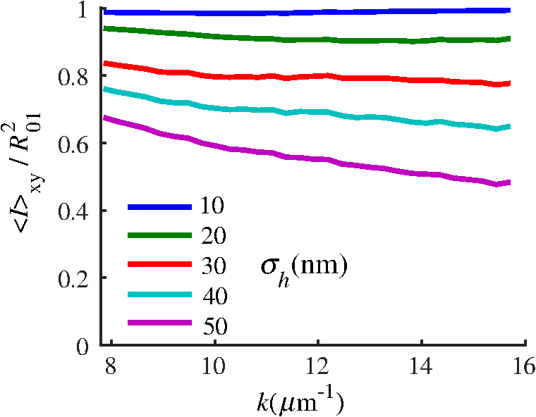

Fig. 15

Bright-field epi-illumination microscope images of inhomogeneous samples with $L = 2 μ m$ (a) $l_{c} = 20 nm$ and a smooth surface, (b) $l_{c} = 100 nm$ and a smooth surface, (c) $l_{c} = 100 nm$ and a rough surface with standard deviation of height variations $σ_{h} = 36 nm$ . Corresponding $Σ (x^{'}, y^{'})$ images, (d) $l_{c} = 20 nm$ and a smooth surface, (e) $l_{c} = 100 nm$ and a smooth surface, (f) $l_{c} = 100 nm$ and a rough top surface. $Σ^{'} (x^{'}, y^{'})$ images, obtained after a second-order polynomial subtraction from detected spectra, are shown in panels (g)–(i) correspondingly. (j) Example spectra for $l_{c} = 20 nm$ smooth (black), $l_{c} = 100 nm$ smooth (red), and $l_{c} = 100 nm$ rough (blue). (k) Average $\tilde{Σ}$ and for the above samples, 10 samples per statistical condition. (l) Average ${\tilde{Σ}}^{'}$ and for the above samples, 10 samples per statistical condition eighth error bars corresponding to standard deviations. Scale bar 300 nm on all panels.

In order to quantify the RI fluctuations within the rough sample, the detected reflectance spectrum undergoes simple postprocessing to remove the effect of nanoscale roughness: (i) $R (x^{'}, y^{'}, k)$ is computed as a second-order polynomial fit to the detected spectrum $I (x^{'}, y^{'}, k)$ , (ii) the fluctuating part of the reflectance intensity is obtained as $δ I (x^{'}, y^{'}, k) = [I (x^{'}, y^{'}, k) - R (x^{'}, y^{'}, k)] / \sqrt{R (x^{'}, y^{'}, k)}$ (transmission coefficients $t_{01}$ and $t_{10}$ are neglected here as they $≊ 1$ ), and (iii) $Σ^{'} (x^{'}, y^{'})$ that is independent of sample surface properties is calculated as the standard deviation of $δ I (x^{'}, y^{'}, k)$ . Physically, the newly introduced parameter $Σ^{'}$ is a measure of nanoscale organization within the sample equivalent to the previously described $\tilde{Σ}$ . However, unlike $\tilde{Σ}$ , $Σ^{'}$ is calculated not simply as standard deviation of detected spectra, but rather the standard deviation of the surface-independent fluctuating part $[I (x^{'}, y^{'}, k) - R (x^{'}, y^{'}, k)] / \sqrt{R (x^{'}, y^{'}, k)}$ which is here necessitated due to surface roughness.

Figure 15 shows illustration to the established ability of the SM technique to quantify structural differences at deeply subdiffractional scales within samples with smooth as well as rough surfaces. Thus, while structural composition within the inhomogeneous samples is impossible to assess from their bright-field microscope images [Figs. 15(a)–15(c)], panels (d) and (e) illustrate that $Σ$ can quantify subdiffractional differences inside smooth samples, and panels (e) and (f) show that $Σ (x, y)$ is affected by surface roughness. Meanwhile, figures in panels (g)–(i) confirm the ability of $Σ^{'} (x, y)$ to measure changes in internal-only sample structure, independent of their surface features. The influence of $l_{c}$ (amplitude of spectral oscillations) and surface roughness (additional low-frequency component creating an overall “tilt” to the spectrum) on SM spectra are shown in panel (j).

4.3.

Comparing Samples with Different $L$

As seen in Eq. (10), $\tilde{Σ}$ depends on sample thickness $L$ , and when an SM signal is acquired from samples with different values of $L$ , $\tilde{Σ}$ may not accurately quantify the differences in the internal-only organization within those samples [Fig. 17(a)]. Thus, in order to quantify the internal structure of a sample, $\tilde{Σ}$ must be normalized by $\sqrt{k_{c} L}$ . Note that the expected value of spectral variance normalized by the unitless parameter $k_{c} L$ is the integral of the PSD tail of sample’s internal organization with known prefactors determined by the instrument setup (NA, $k_{c}$ , $Δ k$ ) and sample geometry ( $R$ ):

Eq. (22)

{\tilde{Σ}}^{2} / k_{c} L = \frac{R k_{c}}{Δ k} \int_{T_{3 D}} ϕ_{n_{Δ}} (k) d^{3} k .

Importantly, when

l_{c}

is on the order of or below

1 / k_{c}

,

\tilde{Σ}

can be approximated to be proportional to

\sqrt{l_{c}}

[coefficient of determination of linear regressions for

\tilde{Σ} (\sqrt{l_{c}})

for

L

between 0.5 and

4 μ m

range from 0.95 to 0.98], hence it allows to quantify the structure of the sample in terms of a physical rather than spectral measure. We here quantify the degree of inhomogeneity inside the sample in terms of the “disorder strength”

L_{d}

of the RI fluctuations inside the sample, defined as the LS of RI variations scaled by the variance of those variations

L_{d} = σ_{n_{Δ}}^{2} l_{c}

. While the explicit relation between

\tilde{Σ}

and

σ_{n_{Δ}}^{2} l_{c}

is complex [Eq. (20)],

L_{d}

can be approximated as

Eq. (23)

L_{d} = σ_{n_{Δ}}^{2} l_{c} \approx A \frac{{\tilde{Σ}}^{2}}{k_{0} {NA}^{2} k_{c} L R},

where

A = 20.7

is a dimensionless proportionality constant,

k_{0}

is the central wavenumber evaluated in vacuum

k_{0} = k_{c} / n_{1}

, and

Δ k_{0}

is the bandwidth of light evaluated in vacuum (hence sample-independent). Comparison between true

L_{d}

and that predicted from an SM measurement

\tilde{Σ}

according to Eq. (23) is shown in Fig. 16(a). Transition from

\tilde{Σ}

to

L_{d}

for samples with very different thicknesses and nanoscale correlation lengths is illustrated in Fig. 17.

Fig. 16

(a) Comparison between true $L_{d}$ and that predicted from an SM measurement $\tilde{Σ}$ for samples with various thickness values ranging from 0.5 to $4 μ m$ . (b) Comparison between true $D$ and that predicted from an SM measurement $\tilde{Σ}$ for samples with $L$ from 0.5 to $4 μ m$ , $L_{n} = 1 μ m$ (solid lines), and $L_{n} = 2 μ m$ (dashed lines).

Fig. 17

Finding $L_{d} = l_{c} σ_{n_{Δ}}^{2}$ from $\tilde{Σ}$ for samples with nanoscale $l_{c}$ of 20 and 60 nm and very different thicknesses.

An alternative way to define the disorder strength is $σ_{n_{Δ}} l_{c}$ , which can be predicted from $\tilde{Σ}$ as $σ_{n_{Δ}} l_{c} \approx A_{1} \tilde{Σ} / (k_{0} NA \sqrt{k_{c} L} \sqrt{R})$ with $A_{1} = 1.8$ . While this relation is more accurate than that in Eq. (23) ( $R^{2} \geq 0.99$ , $L$ between 0.5 and $4 μ m$ as above) and has been utilized in previous works,⁴¹^–⁴³ it is only valid for a smaller range of structural LSs $x < 0.5$ .

Finally, for fractal media $\tilde{Σ}$ can also be used to measure the fractal dimension $D$ of sample organization. While the explicit analytical relation between $\tilde{Σ}$ and $D$ given in Eq. (19) is quite complex, for fractal media $\tilde{Σ}$ is linearly proportional to both $D$ [ $D \in (2,3)$ , Figs. 4(a) and 4(b)] and $σ_{n_{Δ}}$ , therefore, a simplified empirical expression can be obtained. For samples with $L > 2 μ m$ , the fractal dimension in combination with the standard deviation of RI can be predicted from $\tilde{Σ}$ measured by SM as

Eq. (24)

σ_{n_{Δ}} (D - D_{0}) = B \frac{\tilde{Σ}}{NA \sqrt{k_{c} L R}},

where

B

is a unitless proportionality constant

B = 13.2

, and

D_{0}

is a fractal dimension offset

D_{0} = 1.33

, which, incidentally, equals the fractal dimension of a 2-D polymer. Figure 16(b) shows the predictions of

σ_{n_{Δ}} (D - D_{0})

from

\tilde{Σ}

for samples with different thicknesses, also confirming the lack of their dependence on

L_{n}

. Based on Eq. (19),

\tilde{Σ} / \sqrt{k_{c} L}

becomes independent of

L

when thickness is large, as a result of which

σ_{n_{Δ}} (D - D_{0})

predictions converge to their true theoretical values. For

L < 2 μ m

, in turn, the predicted

σ_{n_{Δ}} (D - D_{0})

is still a monotonic function of the theoretical, but overestimates its true value.

Importantly, while the above relations are shown on examples of exponential or fractal RI SCFs, an arbitrary correlation function can always be described through the effective correlation length $l_{c}^{eff}$ , defined as separation distance at which correlation decays by a factor of $e$ . In this case, the relation $\tilde{Σ} \propto σ_{n_{Δ}} \sqrt{l_{c}^{eff}}$ still holds (as illustrated in Fig. 4), and the spatial distribution of material can still be described through $L_{d} = σ_{n_{Δ}}^{2} l_{c}^{eff}$ . The monotonic relation between the fractal dimension $D$ and the effective correlation length $l_{c}^{eff}$ is shown in Fig. 18.

Fig. 18

Increase in the effective correlation length $l_{c}^{eff}$ with the fractal dimension $D$ . Here, $L_{n} = 1 μ m$ .

In summary, to measure the structural characteristic $L_{d}$ of purely internal nanoscale organization of complex, weakly scattering samples, one needs to measure $\tilde{Σ}$ as well as the sample’s optical thickness with respect to central wavenumber $k_{c} L$ . To measure a sample’s optical thickness, a range of techniques can be employed. Methodologies for measuring a sample’s physical thickness (which necessitates an assumption of sample’s RI) include atomic force microscopy and optical interference-based optical profilometry.⁴⁴ At the same time, a sample’s optical thickness can be measured via a range of quantitative phase microscopy (QPM) techniques as reviewed in Refs. 45 and 46. Regarding the QPM techniques, we note that the QPM feature could not be combined with our instrument since an altered incident light path would be required along with transmission-mode light collection scheme. Below, we review two methods for obtaining a sample’s optical thickness from SM-registered signal itself, with no need for additional instrumentation or data acquisition steps.

As follows from Eq. (6), the classical SM spectrum consists of a deterministic zero-frequency offset and a fluctuating component $δ I (k)$ . The highest spectral frequency in the fluctuating component $δ I (k)$ corresponds to the interference between the waves reflected at $z = 0$ and $z = - L$ , with the corresponding optical path difference (OPD) between the two waves equal to $OPD = 2 n_{1} L$ . Thus, the optical thickness $n_{1} L$ of the sample can be measured by taking the Fourier transform of the fluctuating component of registered SM spectrum $F {δ I (k)} = \tilde{I} (z)$ evaluating the highest spectral frequency of the measured signal.

Note that the accurate measurement of sample optical thickness given the sample geometry required by the SM technique (RI match at one interface) is complicated by the fact that sample–substrate interface does not always reflect light due to the low RI contrast at the bottom interface typical to fixed biomaterials on glass slides. Specifically, this is the case when $l_{c}$ is smaller than the diffraction-limited spot and the frequency-space spectrum ${\tilde{I}}^{2} (z)$ does not necessarily contain an evident peak at $z = - L$ . Nevertheless, the spectral-frequency composition of the SM signal can be analyzed to extract thickness without the need for additional instrumentation or data acquisition steps. Below, we review two methods for sample thickness evaluation from an SM signal (a) based on the decay rate of the autocorrelation of the fluctuating component $δ I (k)$ ,⁴¹^,⁴³ and (b) based on the shape of the frequency-space spectrum $\tilde{I} (z)$ .²³

4.3.1.

Spectral correlation decay rate

One way to measure $L$ is through the autocorrelation of the registered SM spectrum. Let the autocorrelation function of $δ I (k)$ be defined as $B_{δ I} (δ k)$ . Then by definition, the correlation decay rate (CDR) is

Eq. (25)

CDR = - \lim_{δ k \to 0} \frac{\ln [B_{δ I} (δ k)]}{δ k^{2}},

where ln denotes a natural logarithm. Since

δ k

is small, this calculation of CDR is equivalent to performing Taylor series expansion of

B_{δ I} (δ k)

around

δ k \approx 0

, and extracting the coefficient of the quadratic term. The Taylor expansion of

B_{δ I} (δ k)

around

δ k \approx 0

can be conveniently evaluated through

\tilde{I} (z)

using the definitions of the Fourier transform and an autocorrelation function:

Eq. (26)

B_{δ I} (δ k) \overset{δ k \to 0}{\overset{}{=}} \frac{\int {| \tilde{I} (z) |}^{2} \frac{1}{2} δ k^{2} z^{2} d z}{\int {| \tilde{I} (z) |}^{2} d z} .

Thus, substituting Eq. (26) into the definition of CDR in Eq. (25), we find

Eq. (27)

CDR = \frac{\int {| \tilde{I} (z) |}^{2} z^{2} d z}{2 \int {| \tilde{I} (z) |}^{2} d z} .

In other words, CDR is the second moment of the Fourier transform of reflectance intensity spectrum

δ I (x, y, k)

. Note that this means CDR is most affected by the highest spectral frequencies of the spectrum, which explain its further described high sensitivity to noise.

Equation (27) simplifies the understanding of how CDR depends on $n_{1} L$ . Depending on the shape of $\tilde{I} (z)$ , CDR in a noiseless system can be anywhere from ${(n_{1} L)}^{2} / 6$ [scattering probability is same for all $z$ and $\tilde{I} (z)$ can be approximated as a top hat function] to $2 {(n_{1} L)}^{2}$ [simple thin-film interference, with $\tilde{I} (z)$ being a delta-function $δ (z - 2 n_{1} L)$ ].

In realistic systems where detector noise is present, $\tilde{I} (z)$ has noise contributions at all depths $z$ , and CDR becomes a complex function of $L$ , SNR, the type and cutoff of low-pass filter used to eliminate spectral noise, as well as the spectral resolution bandwidth of the detector. In simple terms, this dependence can be explained as follows: after low-pass filtration of the detected spectrum, noise contributions to $\tilde{I} (z)$ at $z > L_{f}$ are eliminated, and CDR is expressed as

Eq. (28)

CDR = \frac{2 A {\tilde{Σ}}^{2} {(n_{1} L)}^{2} + \frac{1}{3} N^{2} L_{f}^{2}}{2 ({\tilde{Σ}}^{2} + N^{2})},

where

N^{2}

is the total power of noise oscillations, and

L_{f}

is found as

λ_{c}^{2} / δ λ_{noise}

with

λ_{c}^{2}

denoting the central wavelength of spectral bandwidth,

δ λ_{noise}

denoting the width of the wavelength interval at which noise oscillations can occur. In general,

δ λ_{noise}

is a combination of the width of the low-pass filter cutoff in the wavelength space

δ λ_{filt}

and the spectral resolution of the detector

δ λ_{\det}

,

δ λ_{noise} = \sqrt{(δ λ_{\det}^{2} + δ λ_{filt}^{2}) / 2}

.

Defining SNR as $SNR = \tilde{Σ} / N$ , we obtain

Eq. (29)

CDR = \frac{A {(n_{1} L)}^{2} + \frac{1}{6 {SNR}^{2}} L_{f}^{2}}{1 + 1 / {SNR}^{2}} .

For a case with

δ λ_{\det} = 1 nm

,

δ λ_{filt} = 12.5 nm

,

λ_{c} = 600 nm

, based on rigorous FDTD simulations of a physical experiment, for samples with a wide range of internal RI distribution properties (i.e.,

l_{c}

between 20 and 250 nm), thickness can be found from CDR simply as

Eq. (30)

L = \sqrt{CDR} / (0.7 n_{1}) - 0.6 μ m .

Figure 19 shows the accuracy of thickness predicted from CDR according to Eq. (30) for various

L

and SNR, where the value of CDR is evaluated either directly from FDTD-simulated physical experiment [Figs. 19(b) and 19(c)] or theoretically via the Eq. (29) [Fig. 19(c)]. The close match with the CDR values obtained from FDTD simulations of a physical experiment confirm the accuracy of the CDR estimates in the conditions of experimental noise as derived in Eq. (29).

Fig. 19

(a) Example spectrum for $L = 3 μ m$ , $l_{c} = 34 nm$ originally simulated by FDTD (red), with added noise to imitate experimental conditions in the case of poor $SNR = 2$ (cyan), and after applying low-pass frequency filter to remove noise (black dashed). The filtered signal approximates the original with 2% accuracy and is used for further CDR calculations. (b) Thickness predicted from CDR for various SNR (solid lines in red for $L = 3 μ m$ , green for $L = 2 μ m$ , blue for $L = 1 μ m$ ). True sample thickness is indicated by dashed lines of the corresponding color. (c) Thickness predicted from CDR at $SNR = 10$ measured from FDTD-simulated spectra (blue) as well as predicted theoretically (orange) for a wide range of true sample thicknesses.

4.3.2.

Decay of the frequency-space spectrum

Another signal processing algorithm capable of accurate sample thickness measurements at even lower values of SNR utilizes the fact that no light scattering events occur at $z > - L$ , and therefore, the expectation ( $E [\cdot]$ ) of the absolute value of frequency-space spectrum $E [| {\tilde{I}}^{2} (z) |]$ always decays at $| z | > L$ .²³ While the exact shape of $E [| {\tilde{I}}^{2} (z) |]$ decay tail at $| z | > L$ has no closed-form analytical expression, this shape can be quantified and stored numerically using the library if FDTD-simulated data for a range of sample properties.

Since the shape of $| \tilde{I} (z) |$ depends on the RI correlation length $l_{c}$ , a fourth-order polynomial was fitted to all FDTD-calculated frequency-space spectra $E [| \tilde{I} (z) |]$ at $| z | > L$ for samples with 20 values of $l_{c}$ (between 20 and 250 nm), and a library of corresponding polynomial coefficients was stored. Then, the optical thickness of the sample is determined as the $z$ -location corresponding to the best fit between an arbitrary experimentally measured $E [| \tilde{I} (z) |]$ decay and that reconstructed from the stored library of $E [| \tilde{I} (z) |]$ . The excellent accuracy of thickness predicted from the tail of $E [| \tilde{I} (z) |]$ at $| z | > L$ for FDTD-synthesized SM data from sampled with various $L$ and SNR is shown in Fig. 20.

Fig. 20

(a) Example Fourier transform of spectrum for $L = 2 μ m$ , generated by FDTD (blue) and the decay fit (black). (b) Thickness predicted from decay tail for various SNR (solid lines in red for $L = 3 μ m$ , green for $L = 2 μ m$ , blue for $L = 1 μ m$ ). True sample thickness is indicated by dashed lines of the corresponding color. (c) Thickness predicted from decay tail measured from FDTD-simulated spectra for a wide range of true sample thicknesses.

To summarize, optical thickness of a studied sample can be calculated from the SM signal using the frequency content of the registered spectra. One option is to use the decay rate of spectral correlation function, CDR. This method allows accurate thickness predictions for samples thicker than 800 nm [Fig. 19(c)]. In addition, thickness can be predicted for each diffraction-limited spot. The disadvantage of this method lies in the high sensitivity of CDR to the presence of experimental noise: when $SNR < 4$ the thickness predictions become inversely proportional to $\tilde{Σ}$ [Fig. 19(b)].

Another method for thickness reconstruction using an SM signal is based on evaluating $L$ directly from the shape of its Fourier transform. The advantages of this method include the independence of noise floor for $SNR > 1$ and a high accuracy in predicting thickness for samples as thin as 200 nm. However, this method requires calculation of the expected value of the frequency-space spectra, which means that $| \tilde{I} (z) |$ from different diffraction-limited spots needs to be calculated and averaged to yield $E [| \tilde{I} (z) |]$ . Thus, the spatial resolution of thickness determined with this method is $\sim 5 \times 5$ diffraction-limited spots.²³ Other disadvantages of this method stem from the fact that it is based on a curve-fitting, error-minimization algorithm. Thus, in addition to requiring longer computational time, this method can be prone to large errors when the experimental and the theoretical curves do not match well, such as when the experimental sample has microscale roughness, or when due to certain hardware specifics the system’s noise is not white noise.

Finally, Fig. 21 shows the comparison of thickness predictions from a complex, rough experimental sample (tissue biopsy) predicted via CDR [Figs. 21(a) and 21(b)], decay of the frequency-space spectrum [Fig. 21(c)], and an atomic force microscope [Fig. 21(d)].

Fig. 21

$L (x, y)$ of a fixed prostate tissue section ( $μ m$ ) calculated using: (a) thickness reconstruction from CDR considering every pixel independently, and (b) applying a median filter with a window size of a diffraction-limited spot, pixels with SNR $< 1$ excluded, (c) thickness reconstruction using frequency-spectral decay, and (d) atomic force microscopy measurements. Panels c-d reproduced with permission from Ref. 23, courtesy of J. Biomed. Opt.

5. Alternative Markers of Spectroscopic Microscopy

Naturally, the SM microscopy signal can be analyzed in a range of ways. In this paper, we provided an in-depth review of the spectral variance $\tilde{Σ}$ and its measurement of the nanoscale structure within weakly scattering samples. In fact, the disorder strength measured through $\tilde{Σ}$ in the SM-based PWS microscopy technique has proven effective in detecting hallmarks of carcinogenesis in histologically normal-appearing cells, facilitating the development of accurate screening techniques for multiple early stage human cancers, including cancers in lung,¹³^,⁴² colon,⁴¹^,⁴²^,⁴⁷ ovaries,¹⁴ pancreas,⁴² esophagus,¹⁵ and prostate.¹⁶

At the same time, an optical parameter equivalent to $\tilde{Σ}$ can be calculated when the standard deviation of reflectance (at a single wavelength of light) $\tilde{Σ_{p}} (λ)$ is taken across pixels of the registered bright-field microscope image, instead of evaluating it across different wavelengths as reviewed herein.⁴⁸ That is, the standard deviation of reflectance across different realizations of media with same statistical properties (i.e., standard deviation across pixels) is identical to standard deviation of reflectance from the same medium (registered in a single pixel) measured at different wavelengths of light. In general, measuring the spectral standard deviation $Σ (x, y)$ has the advantage of quantifying the sample subvolumes imaged by individual pixels independently and thus not making the assumption of different pixels imaging statistically equivalent samples with similar physical thicknesses. Nevertheless, in cases when samples can be assumed to be statistically homogeneous, evaluation of a sample’s internal properties using few ( $\approx 30$ ) wavelengths of light instead of 200 has the advantage of system speed improvement by orders of magnitudes along with the possibility of obtaining measurements of whole microscopy slides,⁴⁸ both of which have great promise for the translational applications of the technique. The applicability of reduced-wavelength ${\tilde{Σ}}_{p} (λ)$ to a given type of samples can be tested by performing an initial set of full-wavelength $Σ (x, y)$ measurements after which the spatial homogeneity of structural properties within those sample can be evaluated when $\tilde{Σ}$ is compared to ${\tilde{Σ}}_{p}$ .

Another array of possible ways to quantify sample properties is through the frequency decomposition of reflectance spectra, i.e., their Fourier transform. From the physical origin of the SM signal as described by Eq. (6), frequency decomposition allows us to identify the depth inside the sample at which the measured scattering events have occurred (Fig. 20) with a resolution defined by the bandwidth of light. This information can be used in a range of ways, as follows. First, in the case of thick samples with $L > 1 μ m$ the frequency spectrum $\tilde{I} (z)$ can be used with no further postprocessing as means of depth-resolved nanoscale structural quantification. Second, a partial integration of the frequency-scape spectrum can be performed: $Σ_{L_{\min}} = \sqrt{\int_{0}^{L_{\min}} {| \tilde{I} (z) |}^{2} d z}$ , where $L_{\min}$ is the smallest possible thickness for the given sample type. This method avoids the thickness-dependence of measured quantity $Σ_{L_{\min}}$ , as only the scattering events occurring within $z \in (0, - L_{\min})$ are quantified regardless of the true sample thickness. The disadvantage of this method lies in the fact that when reflectance at $z = - L$ is not measured, $Σ_{L_{\min}} \propto Σ_{R}$ [Eq. (14)] which is a nonmonotonic function of the structural LS $l_{c}$ .

Finally, since $\tilde{I} (z)$ conveys the power of light scattered at depth $z$ , it can be used to obtain two independent optical measures of sample structure: ${\tilde{Σ}}_{R}$ (scattering inside the sample) and ${\tilde{Σ}}_{L}$ [scattering at $z = - L$ , Figure 22(a)²³]. Hence, following the known analytical equations for ${\tilde{Σ}}_{R}$ and ${\tilde{Σ}}_{L}$ [Eqs. (18) and (17)], the explicit physical properties of sample structure $l_{c}$ and $σ_{n}$ can be independently calculated [Fig. 22(b)]. The obvious great advantage of this approach lies in measuring nonambiguous, explicit, spatially resolved parameters of sample structure. The disadvantages include the assumption of sample statistical properties being similar at $z = - L / 2$ and $z = - L$ as well as the necessary multistep signal postprocessing algorithm which, given imperfect experimental data, can cause error accumulation.

Fig. 22

(a) ${\tilde{Σ}}_{R} / \sqrt{k_{c} L}$ and ${\tilde{Σ}}_{L}$ as a function of the correlation length $l_{c}$ obtained for a sample with thickness $L = 2 μ m$ according to analytical equations (solid lines) and calculated from FDTD simulation (circles with error bars corresponding to the standard deviation between nine ensembles per statistical condition). (b) Corresponding true $σ_{n_{Δ}}$ and $l_{c}$ (solid lines) and reconstructed from FDTD-synthesized SM signal (circles with error bars corresponding to the standard deviation between nine ensembles per statistical condition). Reproduced with permission from Ref. 23, courtesy of J. Biomed. Opt.

6. Summary and Outlook

Despite the diffraction limit of imaging resolution, the second-order statistic of the spectroscopic content of a reflected-light bright-field microscope image contains information about the structural organization within a label-free weakly scattering sample at arbitrarily small length scales, limited only by the SNR rather than by a physical phenomenon. Here, we have reviewed the fundamental principles behind the technique’s LS sensitivity and provided a detailed description of its various aspects. In addition, we discussed the different approaches to data analysis which can be taken depending on the characteristics of studied samples, such as degree of nanoscale surface roughness and sample thicknesses, as well as on how important the spatial resolution of nanoscale information ( $\tilde{Σ} (x, y)$ ) and the speed of data acquisition ( ${\tilde{Σ}}_{p}$ ) are for the particular application. Similarly, some of the instrumentation features can be adjusted to achieve the desired depth of focus, or the sample geometry can be altered to allow measurements from other sample types, such as living biological cells,¹⁸^,⁴⁹ while satisfying the requirements of the technique.

From the instrumentation perspective, the SM technique is quite simple and can even be built into a commercial microscope.¹⁸ A crucial aspect of the technique is the sample geometry. First, it ensures the existence of a reference arm and leads to an SNR ( $\tilde{Σ} \propto σ_{n_{Δ}}$ ) that is much greater than that of methods detecting the intensity of scattered light directly from the sample ( $\propto σ_{n_{Δ}}^{2}$ ). Second, combined with the sample thickness not exceeding the microscope’s depth of field, it defines the nature of SM’s LS sensitivity, as discussed in Sec. 3.2.²¹

Importantly, the unique aspect behind the technology is not the instrument itself, but rather the derived nanoscale-sensitive marker ${\tilde{Σ}}^{2}$ . It offers distinct advantages compared to the textbook optical properties which the common light scattering spectroscopic techniques quantify, such as the backscattering ( $σ_{b}$ ) and the total scattering ( $σ_{s}$ ) cross sections. $σ_{b}$ has a nonmonotonic dependence on $l_{c}$ which makes the inverse problem ambiguous,³⁷ and $σ_{s}$ increases steeply $\propto l_{c}^{3}$ and thus is relatively insensitive to structural changes at small length scales.³⁹ $\tilde{Σ}$ , in turn, is a “monotonic” function of the length scale composition of the sample, with its value saturating at large length scales, as a result of which it exhibits a predominant sensitivity to changes at subdiffraction length scales.¹⁹ Finally, as reviewed herein, $\tilde{Σ}$ possesses a unique ability to detect structures at any length scale whatsoever.²¹

The SM approach also clearly differs from other label-free techniques utilizing the spectral content of diffraction-limited microscope images for extracting structural information about the sample. Unlike the high-precision quantitative phase techniques, it measures the fluctuations of RI rather than its longitudinal integral. Compared to subdiffraction-sensitive techniques such as confocal light scattering and absorption spectroscopy,¹ spatial-domain low-coherence QPM,⁸^,⁹ spectral encoding of spatial frequency,²^–⁴ or nanoscale nuclear architecture mapping,¹⁰ the theory behind SM¹ does not impose strong assumptions such as approximation of the medium as solid spheres or having a dominant length scale² and provides an explicit relation between the sample’s complex 3-D RI distribution and the derived quantitative measure ${\tilde{Σ}}^{2}$ . This relation is applicable to arbitrary types of RI distribution within the sample: continuous or discrete, random or deterministic, statistically isotropic or not.

SM, with its great advantages for basic science, biology and medical applications, enables quantitative assessment of the microscopically indiscernible, nanoscale structural features of optically transparent materials such as biological cells and tissues without the need for external contrast agents. Thus, PWS microscopy utilizes SM to detect intracellular structural alterations preceding tumor formation both for the development of early cancer screening methodology,¹⁷ and for basic biology studies of the mechanisms behind tumor-specific intracellular alterations as well as their effect on gene regulation.⁵⁰ Prospects for the reviewed technique also include identification of new cancer therapeutics by offering intracellular ultrastructure-based approach to screen drugs for their ability to revert malignancy-associated changes. In addition, the relatively simple instrumentation requirements open the door to a wide range of possible directions for further technology development. This includes a high-throughput automated whole-slide SM approach complementing highly effective tools such as whole-slide microscopy and digital pathology, sample geometry alterations to allow both structural and temporal data acquisition from live biological cells, as well as implementation of confocal, structural, or other illumination techniques to obtain axially resolved, 3-D cubes of the nanoscale-sensitive marker $\tilde{Σ}$ or the explicit parameters such as RI correlation length and variance.

Disclosures

Dr. Subramanian and Dr. Backman are cofounders and/or shareholders in Nanocytomics LLC.

Acknowledgments

This study was supported by the National Institutes of Health under Grant Nos: R01CA200064, R01CA155284, R01CA165309, R01EB016983, and U54CA193419, and by the National Science Foundation under Grant No. CBET-1240416, and by the Lungevity Foundation. The FDTD simulations were made possible by a computational allocation from the quest high-performance computing facility at Northwestern University.

References

1.

I. Itzkan et al., “Confocal light absorption and scattering spectroscopic microscopy monitors organelles in live cells with no exogenous labels,” Proc. Natl. Acad. Sci. U. S. A., 104 (44), 17255 –17260 (2007). http://dx.doi.org/10.1073/pnas.0708669104 Google Scholar

2.

S. A. Alexandrov et al., “Spectral encoding of spatial frequency approach for characterization of nanoscale structures,” Appl. Phys. Lett., 101 (3), 033702 (2012). http://dx.doi.org/10.1063/1.4737209 APPLAB 0003-6951 Google Scholar

3.

S. Alexandrov and D. Sampson, “Spatial information transmission beyond a system’s diffraction limit using optical spectral encoding of the spatial frequency,” J. Opt. A: Pure Appl. Opt., 10 (2), 025304 (2008). http://dx.doi.org/10.1088/1464-4258/10/2/025304 Google Scholar

4.

S. A. Alexandrov et al., “Novel approach for label free super-resolution imaging in far field,” Sci. Rep., 5 13274 (2015). http://dx.doi.org/10.1038/srep13274 Google Scholar

5.

C. Joo et al., “Spectral-domain optical coherence phase microscopy for quantitative phase-contrast imaging,” Opt. Lett., 30 (16), 2131 –2133 (2005). http://dx.doi.org/10.1364/OL.30.002131 OPLEDP 0146-9592 Google Scholar

6.

M. A. Choma et al., “Spectral-domain phase microscopy,” Opt. Lett., 30 (10), 1162 –1164 (2005). http://dx.doi.org/10.1364/OL.30.001162 OPLEDP 0146-9592 Google Scholar

7.

M. T. Rinehart, V. Jaedicke and A. Wax, “Quantitative phase microscopy with off-axis optical coherence tomography,” Opt. Lett., 39 (7), 1996 –1999 (2014). http://dx.doi.org/10.1364/OL.39.001996 OPLEDP 0146-9592 Google Scholar

8.

P. Wang et al., “Spatial-domain low-coherence quantitative phase microscopy for cancer diagnosis,” Opt. Lett., 35 (17), 2840 –2842 (2010). http://dx.doi.org/10.1364/OL.35.002840 OPLEDP 0146-9592 Google Scholar

9.

S. Uttam et al., “Investigation of depth-resolved nanoscale structural changes in regulated cell proliferation and chromatin decondensation,” Biomed. Opt. Express, 4 (4), 596 –613 (2013). http://dx.doi.org/10.1364/BOE.4.000596 BOEICL 2156-7085 Google Scholar

10.

S. Uttam et al., “Early prediction of cancer progression by depth-resolved nanoscale mapping of nuclear architecture from unstained tissue specimens,” Cancer Res., 75 (22), 4718 –4727 (2015). http://dx.doi.org/10.1158/0008-5472.CAN-15-1274 CNREA8 0008-5472 Google Scholar

11.

H. Roy et al., “Association between rectal optical signatures and colonic neoplasia: Potential applications for screening,” Cancer Res., 69 (10), 4476 –4483 (2009). http://dx.doi.org/10.1158/0008-5472.CAN-08-4780 Google Scholar

12.

D. Damania et al., “Nanocytology of rectal colonocytes to assess risk of colon cancer based on field cancerization,” Cancer Res., 72 (11), 2720 –2727 (2012). http://dx.doi.org/10.1158/0008-5472.CAN-11-3807 Google Scholar

13.

H. K. Roy et al., “Optical detection of buccal epithelial nanoarchitectural alterations in patients harboring lung cancer: implications for screening,” Cancer Res., 70 (20), 7748 –7754 (2010). http://dx.doi.org/10.1158/0008-5472.CAN-10-1686 CNREA8 0008-5472 Google Scholar

14.

D. Damania et al., “Insights into the field carcinogenesis of ovarian cancer based on the nanocytology of endocervical and endometrial epithelial cells,” Int. J. Cancer, 133 1143 –1152 (2013). http://dx.doi.org/10.1002/ijc.v133.5 IJCNAW 1097-0215 Google Scholar

15.

V. J. Konda et al., “Nanoscale markers of esophageal field carcinogenesis: potential implications for esophageal cancer screening,” Endoscopy, 45 983 –988 (2013). http://dx.doi.org/10.1055/s-00000012 ENDCAM Google Scholar

16.

H. K. Roy et al., “Nanocytological field carcinogenesis detection to mitigate overdiagnosis of prostate cancer: a proof of concept study,” PLoS One, 10 e0115999 (2015). http://dx.doi.org/10.1371/journal.pone.0115999 POLNCL 1932-6203 Google Scholar

17.

H. Subramanian et al., “Procedures for risk-stratification of lung cancer using buccal nanocytology,” Biomed. Opt. Express, 7 (9), 3795 –3810 (2016). http://dx.doi.org/10.1364/BOE.7.003795 BOEICL 2156-7085 Google Scholar

18.

L. M. Almassalha et al., “Label-free imaging of the native, living cellular nanoarchitecture using partial-wave spectroscopic microscopy,” Proc. Natl. Acad. Sci. U. S. A., 113 (42), E6372 –E6381 (2016). http://dx.doi.org/10.1073/pnas.1608198113 Google Scholar

19.

L. Cherkezyan et al., “Interferometric spectroscopy of scattered light can quantify the statistics of subdiffractional refractive-index fluctuations,” Phys. Rev. Lett., 111 033903 (2013). http://dx.doi.org/10.1103/PhysRevLett.111.033903 PRLTAO 0031-9007 Google Scholar

20.

J. Yi and V. Backman, “Imaging a full set of optical scattering properties of biological tissue by inverse spectroscopic optical coherence tomography,” Opt. Lett., 37 (21), 4443 –4445 (2012). http://dx.doi.org/10.1364/OL.37.004443 OPLEDP 0146-9592 Google Scholar

21.

L. Cherkezyan, H. Subramanian and V. Backman, “What structural length scales can be detected by the spectral variance of a microscope image?,” Opt. Lett., 39 (15), 4290 –4293 (2014). http://dx.doi.org/10.1364/OL.39.004290 OPLEDP 0146-9592 Google Scholar

22.

J. Yi et al., “Can OCT be sensitive to nanoscale structural alterations in biological tissue?,” Opt. Express, 21 (7), 9043 –9059 (2013). http://dx.doi.org/10.1364/OE.21.009043 OPEXFF 1094-4087 Google Scholar

23.

L. Cherkezyan et al., “Reconstruction of explicit structural properties at the nanoscale via spectroscopic microscopy,” J. Biomed. Opt., 21 (2), 025007 (2016). http://dx.doi.org/10.1117/1.JBO.21.2.025007 JBOPFO 1083-3668 Google Scholar

24.

D. Cook, Cellular Pathology: An Introduction to Techniques and Applications, 67 –104 Scion, Bloxham (2006). Google Scholar

25.

G. C. Crossmon, “Mounting media for phase microscope specimens,” Stain Technol., 24 241 –247 (1949). http://dx.doi.org/10.3109/10520294909139615 STTEAW 0038-9153 Google Scholar

26.

H. G. Davies et al., “The use of the interference microscope to determine dry mass in living cells and as a quantitative cytochemical method,” J. Cell Sci., 3 (31), 271 –304 (1954). Google Scholar

27.

J. D. Rogers et al., “Modeling light scattering in tissue as continuous random media using a versatile refractive index correlation function,” IEEE J. Sel. Top. Quantum Electron., 20 (2), 173 –186 (2014). http://dx.doi.org/10.1109/JSTQE.2013.2280999 Google Scholar

28.

P. Guttorp and T. Gneiting, “On the Whittle-Matérn correlation family,” Seattle, Washington (2005). Google Scholar

29.

A. Bancaud et al., “A fractal model for nuclear organization: current evidence and biological implications,” Nucl. Acids Res., 40 (18), 8783 –8792 (2012). http://dx.doi.org/10.1093/nar/gks586 Google Scholar

30.

D. Lebedev et al., “Structural hierarchy of chromatin in chicken erythrocyte nuclei based on small-angle neutron scattering: fractal nature of the large-scale chromatin organization,” Crystallogr. Rep., 53 (1), 110 –115 (2008). http://dx.doi.org/10.1134/S1063774508010136 Google Scholar

31.

D. Lebedev et al., “Fractal nature of chromatin organization in interphase chicken erythrocyte nuclei: DNA structure exhibits biphasic fractal properties,” FEBS Lett., 579 (6), 1465 –1468 (2005). http://dx.doi.org/10.1016/j.febslet.2005.01.052 FEBLAL 0014-5793 Google Scholar

32.

L. Cherkezyan et al., “Nanoscale changes in chromatin organization represent the initial steps of tumorigenesis: a transmission electron microscopy study,” BMC Cancer, 14 (1), 189 (2014). http://dx.doi.org/10.1186/1471-2407-14-189 BCMACL 1471-2407 Google Scholar

33.

O. Nadiarnykh et al., “Alterations of the extracellular matrix in ovarian cancer studied by second harmonic generation imaging microscopy,” BMC Cancer, 10 94 (2010). http://dx.doi.org/10.1186/1471-2407-10-94 BCMACL 1471-2407 Google Scholar

34.

S. L. Jacques, C. Alter and S. A. Prahl, “Angular dependence of HeNe laser light scattering by human dermis,” Lasers Life Sci., 1 (4), 309 –333 (1987). Google Scholar

35.

A. J. Radosevich et al., “Subdiffusion reflectance spectroscopy to measure tissue ultrastructure and microvasculature: model and inverse algorithm,” J. Biomed. Opt., 20 (9), 097002 (2015). http://dx.doi.org/10.1117/1.JBO.20.9.097002 JBOPFO 1083-3668 Google Scholar

36.

M. Born and E. Wolf, Principles of Optics, Cambridge University Press, Cambridge, England (1998). Google Scholar

37.

A. Ishimaru, Wave Propagation and Scattering in Random Media, Wiley, Hoboken, New Jersey (1999). Google Scholar

38.

J. Goodman, Introduction To Fourier Optics, Roberts & Co., Englewood, Colorado (2005). Google Scholar

39.

A. J. Radosevich et al., “Structural length-scale sensitivities of reflectance measurements in continuous random media under the born approximation,” Opt. Lett., 37 5220 –5222 (2012). http://dx.doi.org/10.1364/OL.37.005220 OPLEDP 0146-9592 Google Scholar

40.

D. Zhang et al., “Spectroscopic microscopy can quantify the statistics of subdiffractional refractive-index fluctuations in media with random rough surfaces,” Opt. Lett., 40 4931 –4934 (2015). http://dx.doi.org/10.1364/OL.40.004931 OPLEDP 0146-9592 Google Scholar

41.

H. Subramanian et al., “Optical methodology for detecting histologically unapparent nanoscale consequences of genetic alterations in biological cells,” Proc. Natl. Acad. Sci. U. S. A., 105 (51), 20118 –20123 (2008). http://dx.doi.org/10.1073/pnas.0804723105 Google Scholar

42.

H. Subramanian et al., “Nanoscale cellular changes in field carcinogenesis detected by partial wave spectroscopy,” Cancer Res., 69 (13), 5357 –5363 (2009). http://dx.doi.org/10.1158/0008-5472.CAN-08-3895 CNREA8 0008-5472 Google Scholar

43.

H. Subramanian et al., “Partial-wave microscopic spectroscopy detects subwavelength refractive index fluctuations: an application to cancer diagnosis,” Opt. Lett., 34 518 –520 (2009). http://dx.doi.org/10.1364/OL.34.000518 OPLEDP 0146-9592 Google Scholar

44.

G. Makosch and B. Drollinger, “Surface profile measurement with a scanning differential ac interferometer,” Appl. Opt., 23 4544 –4553 (1984). http://dx.doi.org/10.1364/AO.23.004544 APOPAI 0003-6935 Google Scholar

45.

G. Popescu, “Quantitative phase imaging of nanoscale cell structure and dynamics,” Methods Cell Biol., 90 87 –115 (2008). http://dx.doi.org/10.1016/S0091-679X(08)00805-4 MCBLAG 0091-679X Google Scholar

46.

M. Mir et al., “Quantitative phase imaging,” Prog. Opt., 57 133 –217 (2012). http://dx.doi.org/10.1016/B978-0-44-459422-8.00003-5 POPTAN 0079-6638 Google Scholar

47.

D. Damania et al., “Nanocytology of rectal colonocytes to assess risk of colon cancer based on field cancerization,” Cancer Res., 72 (11), 2720 –2727 (2012). http://dx.doi.org/10.1158/0008-5472.CAN-11-3807 CNREA8 0008-5472 Google Scholar

48.

J. E. Chandler et al., “Nanoscale refractive index fluctuations detected via sparse spectral microscopy,” Biomed. Opt. Express, 7 883 –893 (2016). http://dx.doi.org/10.1364/BOE.7.000883 BOEICL 2156-7085 Google Scholar

49.

L. M. Almassalha et al., “Basis microscopy: label-free imaging of the native, living cellular nano-architecture,” FASEB J., 30 (1 Suppl.), 780 –783 (2016). FAJOEC 0892-6638 Google Scholar

50.

L. M. Almassalha et al., “The global relationship between chromatin physical topology, fractal structure, and gene expression,” Sci. Rep., 7 41061 (2016). https://doi.org/10.1038/srep41061 Google Scholar

Biography

Lusik Cherkezyan is a postdoctoral fellow in the Department of Biomedical Engineering, Northwestern University, Evanston, Illinois, USA, where she has also received her PhD. Her work focuses on the use of physics and engineering principles to the study of biological systems. In particular, she is interested in technology development for the spectroscopic quantification of biomaterials at nanometer scales. Her work has been published in multiple high-profile journals, including Physical Review Letters, BMC Cancer, Optics Letters, Endoscopy, etc.

Di Zhang received his BS degree in electrical engineering from Beijing Jiaotong University, China, in 2009. He is currently working toward his PhD in biomedical engineering at the Northwestern University, Evanston, Illinois, USA. His research interests include computational electromagnetics for modeling light interaction with biological tissue and optical imaging techniques for early stage cancer detection.

Hariharan Subramanian received his PhD in biomedical engineering from Northwestern University, where he is currently a research professor of biomedical engineering. He is the cofounder and chief technology officer of NanoCytomics, an in vitro medical diagnostic company developing screening strategies for different types of cancers (e.g., lung, colon, prostate, etc.). He has considerable experience in biomedical optics, cancer biology, and clinical research, with numerous publications appearing in leading peer-reviewed journals.

Ilker Capoglu received his PhD from the School of Electrical and Computer Engineering at Georgia Institute of Technology in 2007. Since 2014, he has been served as a local Houston manager and scientific advisor for the Electromagnetics Sensor Physics Group at Halliburton. He has authored 21 peer-reviewed publications in high profile journals such as Progress in Optics, IEEE TAP, Physics Review Letters, and PNAS. He is the principal developer of a comprehensive numerical electromagnetics software package (“Angora”).

Allen Taflove is a professor in the Department of Electrical Engineering and Computer Science, Northwestern University, Evanston, Illinois, USA. Since 1972, he has pioneered finite-difference time-domain (FDTD) computational solutions of Maxwell’s equations, for which he received the 2014 IEEE Electromagnetics Award. His major publication, Computational Electrodynamics: The Finite-Difference Time-Domain Method, is the 7th most-cited book in physics.

Vadim Backman is the Walter Dill Scott professor of biomedical engineering at Northwestern University and a program leader at the Robert H. Lurie Comprehensive Cancer Center in Chicago, Illinois, USA. An internationally renowned expert in biomedical optics, he develops revolutionary nanoscale imaging technologies that allow researchers to explore previously intractable questions in biology, disease diagnosis, and progression, with a focus on detecting cancer at its earliest and most treatable stages.

CC BY: © The Authors. Published by SPIE under a Creative Commons Attribution 4.0 Unported License. Distribution or reproduction of this work in whole or in part requires full attribution of the original publication, including its DOI.

Citation Download Citation

Lusik Cherkezyan, Di Zhang, Hariharan Subramanian, Ilker Capoglu, Allen Taflove, and Vadim Backman "Review of interferometric spectroscopy of scattered light for the quantification of subdiffractional structure of biomaterials," Journal of Biomedical Optics 22(3), 030901 (14 March 2017). https://doi.org/10.1117/1.JBO.22.3.030901

Received: 13 August 2016; Accepted: 20 February 2017; Published: 14 March 2017

Access the abstract

JOURNAL ARTICLE
19 PAGES

DOWNLOAD PAPER SAVE TO MY LIBRARY

GET CITATION

CITATIONS

Cited by 22 scholarly publications.

Explore citations on Lens.org

KEYWORDS

Light scattering

Signal to noise ratio

Spectroscopy

Microscopes

Scattering

Interferometry

Microscopy

Show All Keywords

CHORUS Article. This article was made freely available starting 14 March 2018

1.

Introduction

2.

Theoretical Principles of Spectroscopic Microscopy

Fig. 1

2.1.

Sample Structure

Eq. (1)

Eq. (2)

Fig. 2

Eq. (3)

2.2.

Light Propagation

Eq. (4)

Fig. 3

Eq. (5)

Eq. (6)

2.3.

Quantification of Subdiffraction Length Scales Using Spectroscopic Microscopy

Eq. (7)

Eq. (8)

Eq. (9)

Eq. (10)

Eq. (11)

Eq. (12)

Eq. (13)

Eq. (14)

Eq. (15)

Eq. (16)

Eq. (17)

Eq. (18)

Eq. (19)

Eq. (20)

3.

Length Scale Sensitivity

3.1.

Functional Dependence on the Shape of Spatial Correlation Function

Fig. 4

3.2.

Fundamental Limits to Sizes of Detectable Structures

Fig. 5

Fig. 6

Fig. 7

3.3.

Length Scales Inside Complex Media with the Greatest Contribution to Signal

Eq. (21)

Fig. 8

Fig. 9

Fig. 10

4.

Quantification of Sample’s Internal Organization: Practical Considerations

4.1.

Instrument Design: Numerical Apertures, Light Bandwidth, and Central Wavenumber

Fig. 11

4.1.1.

Magnification

4.1.2.

Illumination Numerical Aperture

Fig. 12

4.1.3.

Collection numerical aperture

Fig. 13

4.1.4.

Wavenumber range Δk

4.1.5.

Central wavenumber kc

Table 1

4.2.

Measurements from Rough Samples

Fig. 14

Fig. 15

4.3.

Comparing Samples with Different L

Eq. (22)

Eq. (23)

Fig. 16

Fig. 17

Eq. (24)

Fig. 18

4.3.1.

Central wavenumber k_c

Comparing Samples with Different $L$