1.

Introduction

Many important biological processes take place inside the cranial bone marrow or just beyond the cranial bone in the brain. Multiphoton excitation microscopy has the potential to acquire deep tissue optical sectioned images with minimal damage in highly scattering media at depths greater than $150\mu \mathrm{m}$.^1–6 This potential has led to widespread use in the bone biology and neuroscience fields. Two-photon microscopy commonly exploits light with longer wavelengths in optimal windows for in vivo tissue imaging (near-IR and IR) with reduced Rayleigh scattering and absorbance to penetrate deeper inside biological tissue; but nonhomogeneous wave propagation through highly scattering turbid media, such as bone, dramatically reduces image resolution even at moderate depths of $\sim 100\mu \mathrm{m}$. In bone, layers of varying refractive index and irregularities in the shape of the matrix produce scattering and refractive optical aberrations that induce phase deviations in the wavefront, which distort the point spread function (PSF) from a diffraction limited imaging system.⁷ A distorted optical wavefront causes the PSF size to increase and its maximum intensity to drop from the ideal, thereby reducing the precision and fidelity of the image.

Several techniques have been proposed to correct such distortions. Optical clearing increases the refractive index homogeneity of the aqueous media and has been effective for imaging collagen⁸ or more recently for a range of tissues using protocols, such as CLARITY.⁹ However, these techniques are only applicable to ex vivo experiments. For in vivo experiments, ablation and thinning of bone improve imaging quality in cranial bone or into the brain^10–13 but induces a biological response to associated tissue damage. An attractive approach to increase imaging resolution in deep tissue for both in vivo and ex vivo imaging without tissue damage is the use of adaptive optics (AO) techniques for microscopy.

AO compensates for tissue-induced distortions using correction element(s) in combination with either a wavefront sensor or image-based sensorless wavefront estimation methods. Wavefront sensor approaches include Shack–Hartmann wavefront sensors with autofluorescent or near-IR guide stars,^14,15 coherence gated wavefront sensing,¹⁶ and image-based methods that use information from acquired images to estimate the wavefront distortions.^17–21 Wavefront sensorless approaches usually estimate an initial error and through an iterative scheme converge to an optimized solution based on metrics, such as total fluorescence intensity for confocal and two-photon microscopy.^22–24 In other microscopy modalities, metrics such as maximum intensity of the image (or a part of the image),²⁵ the low-frequency spatial content of the image, the image sharpness,^26–28 and the Fourier metric²⁹ have been used. To generate a corrected wavefront in all cases, a compensating optical element or elements are required; most commonly deformable mirrors (DM) are used. The correction attainable by a single DM depends on its pitch, number and stroke of actuators, and surface form (segmented or continuous facesheet). This functional characteristic of DMs makes them act as high-pass filters that primarily correct lower order aberrations. For correction of spatially confined high-order aberrations in biological tissues like bone, other technologies such as spatial light modulators (SLMs) or digital micromirror devices (DMDs)^30–32 could potentially assist. They often contain hundreds or thousands of segments, but may have other limitations in response time or correction magnitude.

The most common method for correcting image aberrations for scanning microscopy modalities is by evaluating and compensating for tissue aberrations in multiple spots across the field of view. However, functional limitations tend to reduce the field of view to keep the acquisition and correction speeds reasonable.^33,34 Recently, use of nonlinear guide stars with Shack–Hartmann measurements of wavefront aberrations averaged over a larger area has significantly expanded the corrected lateral field of view to several tens of microns.^15,35 This pragmatic approach yields an accurate measurement of low-order tissue aberrations that has proven useful to extend imaging deep into biological samples, such as the brain.¹⁵ High-order aberrations and scattering that are prevalent in bone change with each focal point, so averaging aberrations from a larger area would limit correction. Therefore, in an alternative wavefront sensorless approach, the adaptive correction element is conjugated to the turbid layer instead of the focus, which improved imaging through bone for a cell-sized field of view.³⁴ To design an AO approach that can effectively correct both low- and high-order aberrations for a larger biologically relevant field of view, it is necessary to characterize the aberrations present in bone, as well as to estimate what portion of those aberrations can be corrected with given deformable element characteristics.

Therefore, in this paper, we investigate the optical aberrations caused by mouse cranial bone. We characterize the bone with experimental data acquired using second-harmonic generation (SHG) imaging in collagen. We simulate the wave propagation in the sample and calculate the amount of wavefront error that can be corrected using a typical commercially available DM, and the residual wavefront error that remains. We further calculate the number of segments a potential second correcting element would require to remove the residual error. Previously, wavefront error measurements have been made in thin biological samples using transmission light microscopy.^36,37 Theoretical³⁸ models of wavefront errors in biological tissue have also been developed. Propagation of electromagnetics wave in biological tissues and cells can be simulated using methods, such as finite-difference time-domain modeling,³⁹ Monte Carlo simulations,⁴⁰ which model radiation transfer, or analytical models.⁴¹ Our work uses a combination of SHG measurements and an analytical approach to model propagation of light through thick sections of highly scattering and randomly structured sections of bone. This fast modeling approach can provide initial information on present optical aberrations for an AO two-photon imaging system, either in open-loop configuration or closed loop. We also calculate the statistics of the different Zernike modes across a large field of view. This work shows that AO correction with a high number of correcting segments could significantly improve resolution when imaging through intact mouse skull.

2.

Methods

2.1.

Theoretical Approach

SHG occurs in noncentrosymmetric crystals, due to redistribution of energy confined in a molecule by a high-energy excitatory laser pulse. This causes symmetric generation of dipole moments, and therefore a noncentrosymmetric polarization signal is produced in one direction. Collagen in bone has a crystalline triple-helix structure that can act as a harmonics generator, and hence frequency up-convertor of light.⁴² The polarization vector can be described in terms of the electric dipole expansion^42–45

Eq. (1)

$$P={\chi }^{(2)}{E}^2,$$

where $P$ is the polarization, $E$ is the electric field, and ${\chi }^{(2)}$ is the second-order nonlinear susceptibility. The intensity of the generated second-harmonic signal $I_{2\omega }$ is proportional to the susceptibility, illumination intensity $I_{\omega }$, pulse duration ${\tau }_p$, and time between pulses ${\tau }_l$ in the form

Eq. (2)

$$I_{2\omega }\propto {({\chi }^{(2)}{I}_{\omega })}^2\frac{{\tau }_l}{{\tau }_p}.$$

The aforementioned equation shows that the SHG signal is the instantaneous response to the laser pulse energy regulated by the second-order susceptibility. We can find a ratio of the refractive index and ${\chi }^{(2)}$, by looking into the molecular structure of the material under study. The value of the second-order susceptibility can be written in terms of the molecular density ${\rho }_m$ and hyperpolarizability $\beta$⁴³

Eq. (3)

$${\chi }^{(2)}={\rho }_m⟨\beta ⟩.$$

The brackets indicate an orientation average. We also have the following ratio between relative permittivity ${ϵ}_r$ and the molecular characteristics of the material

Eq. (4)

$$({ϵ}_r-1){ϵ}_0={\rho }_m⟨\beta ⟩{ϵ}_0.$$

By combining Eqs. (2)–(4) and the relation $n=\sqrt{{ϵ}_r}$, we can express a relation for the refractive index in terms of the SHG signal and laser input energy in the form

Eq. (5)

$$n\propto \sqrt{1+\frac{\sqrt{I_{2\omega }}}{I_{\omega }\sqrt{{\tau }_l/{\tau }_p}}}.$$

We introduce a new parameter $k_1=1/(I_{\omega }\sqrt{{\tau }_l/{\tau }_p})$, and since $k_1\sqrt{I_{2\omega }}$ is a small number, we can use the first-order Taylor expansion

Eq. (6)

$$n\propto 1+\frac{k_1}{2}\sqrt{I_{2\omega }}.$$

Now to account for the proportionality, we substitute an experimentally determined constant for $k_1/2$. We use the background intensity $I_b$ (5% of maximum intensity $I_{\max }$) as a threshold between the SHG signal from the bone and the surrounding medium. The intensities above the threshold are scaled within a range starting from the lower limit of the bone refractive indices $n_{\min }$ and up to $n_{\max }$—which corresponds to $I_{\max }$—and for lower intensities, we assign the refractive index of the immersion medium $n_b$

Eq. (7)

$$n=\{\begin{array}{cc}{k}_2\sqrt{I_{2\omega }-I_b}+n_{\min }& I>I_b\\ n_b& \text{otherwise}\end{array}.$$

Since the intensity of the illumination light is affected by absorption and scattering, we normalize the collected signal intensity for the depth using Beer’s law⁴⁶

Eq. (8)

$$I_{\omega }(z)=I_0\exp (-2z{\mu }_{\mathrm{eff}}),$$

where $z$ is the depth, ${\mu }_{\mathrm{eff}}={\mu }_{\mathrm{a}}+{\mu }_{\mathrm{s}}+{\mu }_{\mathrm{o}}$, and subscripts a, s, and o represent absorption, scattering, and other coefficients, respectively. Factor 2 in the equation accounts for the light propagation forward and backward. Equation (8) is incorporated in the parameter $k$ calculation, such that $k_2(z)=\exp (2z{\mu }_{\mathrm{eff}})k_2(0)$ We use an experimentally determined value of $0.023{\mu \mathrm{m}}^{-1}$ for ${\mu }_{\mathrm{eff}}$, which is within the range found in the literature.^47,48 We acquired three-dimensional (3-D) images of bone using in vivo SHG imaging in the cranial bone from a 3-week-old male wild-type mouse. Each $Z$ slice was produced by averaging 15 frames to increase signal-to-noise ratio. Each SHG image consists of $256\times 256\text{pixels}$ across a $320\mu \mathrm{m}\times 320\mu \mathrm{m}$ field of view. To account for anisotropy of the SHG signal due to fiber orientation in the bone, we acquired stacks of images with transverse polarizations of the input laser ranging from 0 deg to 180 deg at intervals of 15 deg. We used the dataset with the highest average intensity as the input for our simulations. The scaled dataset is shown in Figs. 1(a)–1(c); the average thickness of the sample is $80\mu \mathrm{m}$. A range of indices of refraction from 1.528 to 1.604 with an average of 1.564 was used for the mouse cranial bone,⁴⁹ and a refractive index of 1.33 was used for the $n_b$ of the immersion medium.

Fig. 1

A slice of the refractive-index-mapped dataset of bone structure used for the simulations is shown in (a). 3-D views of the dataset from bottom and top are shown in (b) and (c). The projection volume inside the original SHG dataset is shown in (d) and (e) as the red cone. The cone is exaggerated to better show the projection path. Projections of equally spaced ($l=106\mu \mathrm{m}$) points (blue dots) from the bottom plane in (e) through the red cone are used for simulation. Scale bar in (a) is $50\mu \mathrm{m}$.

3.

Simulations

3.1.

Wavefront Correction Function Calculated by Zernike Polynomials

We used the scaled-to-refractive-index SHG $Z$-stack from mouse cranial bone to calculate the wavefront from a grid of $3\times 3$ equally spaced ($l=106\mu \mathrm{m}$) positions in the bottom plane [Fig. 1(e)]. 51,471 rays on a circle with radius of 128 pixels in Cartesian coordinates were calculated for each projection, yielding a pupil projection that matched the NA-defined cone angle [Figs. 1(d) and 1(e)]. When the phase of the pupil projections was analyzed, pupils out of the center showed tip and tilt predominately due to the angle of off-axis points and curvature of the sample (Fig. 2). We eliminated the tip/tilt due to the off-axis angle, and the projected wavefront in Fig. 2 includes only tip/tilt due to the natural curvature of the skull. We then used these experimental phase values to extract the Zernike coefficients and reconstruct the phase of Zernike functions for each pupil (Fig. 3). The RMS wavefront error values ($\sigma$) [Figs. 3(a)–3(i)] indicate that the bone produces substantial low-order aberrations generated from modes 5 to 37. Therefore, it is likely that low-order aberration correction would improve image quality. However, the difference between the Zernike modeled phase (Fig. 3) and the experimentally measured phase (Fig. 2) suggests that remaining high spatial frequency distortions are important contributors to total image degradation.

Fig. 2

Phase of projected pupils ${\mathrm{\Psi }}_i$ from a $3\times 3$ grid uniformly distributed on the bottom plane of the SHG $Z$-stack in a mouse cranial bone shown in Fig. 1. (a)–(i) correspond to the originating points shown as blue dots in Fig. 1(e). The measured pupils exclude the tip/tilt due to the positions of the originating points with regard to the pupil. Values of RMS wavefront error ($\sigma$) are in radians.

Fig. 3

(a)–(i) Phase of reconstructed wavefronts, generated from the Zernike modes 5 to 37 extracted from projected pupils shown in Figs. 2(a)–2(i), respectively. Color bar values are in radians. RMS wavefront error $\sigma$ of each projection is indicated, respectively.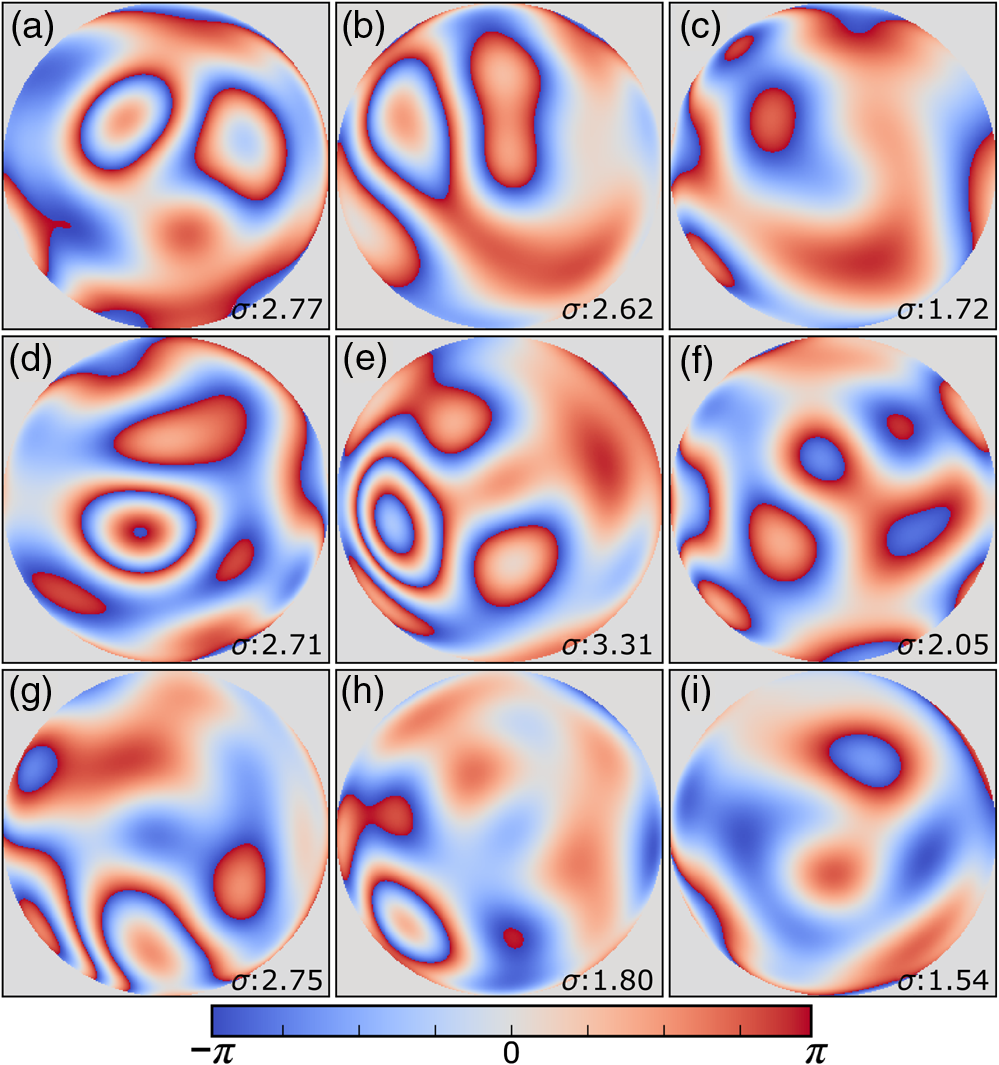

We used these constructed pupils to calculate estimated PSFs in the tissue (Fig. 4). As expected from the calculated wavefront errors, the PSF size is between 1.5 and $10\mu \mathrm{m}$, which is far from the diffraction limit ($\sim 500\mathrm{nm}$ in our case).

Fig. 4

(a)–(i) Normalized PSF calculated from the corresponding wavefronts in Figs. 3(a)–3(i), respectively. Scale bars are $5\mu \mathrm{m}$.

To examine which Zernike modes contributed to the observed PSF degradation, we plotted the coefficients for modes 5 to 37 for each spot in the $3\times 3$ grid (Fig. 5). These values show strong aberrations especially in the lower modes including astigmatism, coma, trefoil, and spherical, which are due to the general shape of the sample. Interestingly, the magnitude of the analyzed modes seems to vary at each point, suggesting differences in bone architecture between each of the analyzed points.

Fig. 5

Zernike modes 5 to 37 corresponding to wavefront shown in Figs. 3(a)–3(i) and PSFs shown in Figs. 4(a)–4(i).

3.2.

Residual Wavefront Error

The calculated pupils and PSFs in the previous sections were all generated from Zernike modes 5 to 37. This essentially results in high-pass filtering of distortions and leaves residual wavefront error that would result in a reduced Strehl ratio for a wavefront corrected system. We calculated the residual wavefront error between the experimental and Zernike modeled pupils such that ${\mathrm{\Psi }}_e={\mathrm{\Psi }}_i/{\mathrm{\Psi }}_c$, which is equivalent to subtracting the phase of the two pupils. We included all of the first 37 Zernike modes (including tip, tilt, and defocus) in our low-order Zernike polynomial aberration pupil modeling, which yielded an understanding of the high-order aberrations that remained in each pupil (Fig. 6). To quantify this residual error, we calculated the root-mean-square error (RMSE) as described by Guo and Wang⁵⁴

Eq. (12)

$${\sigma }_{\mathrm{res}}{=\left\{\frac{{\iint }_A{[{\phi }_i(\mu ,\nu )-{\phi }_c(\mu ,\nu )]}^2\mathrm{d}\mu \mathrm{d}\nu }{{\iint }_A\mathrm{d}\mu \mathrm{d}\nu }\right\}}^{\frac{1}{2}},$$

where $\phi$ is the phase of pupil $\psi$, and $\mu$ and $\nu$ are the coordinates of the pupil plane. RMSE (${\sigma }_{\mathrm{res}}$) was calculated for each residual pupil projection in the $3\times 3$ matrix [Figs. 6(a)–6(i)]. Although a significant amount of aberration was due to low-order Zernike polynomial aberration modeling, additional high-order aberrations remained. This indicates that typical DMs will be unable to correct higher order aberrations important in the bone. Our calculations show that an RMSE of 1.25 radians remains, which indicates that a typical DM is likely to only improve the Strehl ratio to about 20%. This large residual error suggests that wavefront correction solely based on a DM with a low number of actuators for imaging inside or through bone will not fully restore the resolution. The residual error appears to have numerous small high-order aberrations, and therefore either a single corrector with a large number of elements or a second corrector conjugated to a DM with several thousands of segments is required. The values of the RMS errors for all of the pupils are tabulated in Table 1. We also calculated the PSF of the residual errors. Figures 7(a) and 7(b) show a PSF generated from Fig. 6(e), laterally and axially. We fitted a Gaussian curve to the central cross section and found an FWHM of $1.73\mu \mathrm{m}$ after removal of low-order aberrations [Fig. 7(c)].

Fig. 6

Residual wavefront error of the pupils shown in Figs. 2(a)–2(i) that are corrected by the pupils shown in Fig. 3(a)–3(i), respectively. Values of ${\sigma }_{\mathrm{res}}$ are in radians.

Table 1

RMS error values of the original, calculated, and residual pupils are calculated. Strehl ratios corresponding to residual wavefront errors are shown.

	Experimental pupil RMSE	Calculated pupil RMSE		Residual RMSE	Strehl ratio (%) (with residual error)
		Z 1 to 37	Z 5 to 37
U-L (a)	5.44	5.26	2.77	1.32	17.51
U-C (b)	6.70	6.40	2.62	1.92	2.51
U-R (c)	7.01	6.87	1.72	1.25	20.96
M-L (d)	3.78	3.02	2.71	2.07	1.38
M-C (e)	6.35	5.29	3.31	3.11	0.01
M-R (f)	7.61	7.41	2.05	1.64	6.79
D-L (g)	7.31	7.10	2.75	1.62	7.25
D-C (h)	8.04	7.87	1.80	1.53	9.62
D-R (i)	8.99	8.89	1.54	1.25	20.96

Note: U, M, and D represent up, middle, and down rows, respectively, and L, C, and R represent left, center, and right columns, respectively. Except Strehl ratios, all other values are in radians.

Fig. 7

PSF after low-order correction. (a) Shows a PSF generated from Fig. 6(e). An axial cross section is shown in (b). Plot of the central cross section of (a) is shown in (c). Scale bars are $5\mu \mathrm{m}$.

To find the number of segments required for effective correction of the residual wavefront error, we calculate its correlation length, to find the smallest aberrated distance, from which we can calculate the number of segments. We first calculate the autocorrelation of the residual wavefront error for each pupil with itself, normalized by the residual RMSE⁵⁵

Eq. (13)

$$\gamma (\mathrm{\Delta }\mu ,\mathrm{\Delta }\nu )=\frac{{\iint }_A{\phi }_e(\mu ,\nu ){\phi }_e(\mu -\mathrm{\Delta }\mu ,\nu -\mathrm{\Delta }\nu )\mathrm{d}\mathrm{\Delta }\mu \mathrm{d}\mathrm{\Delta }\nu }{{\sigma }_{\mathrm{res}}^2}.$$

Using the calculated autocorrelation, we can then find the correlation length $\mathrm{\Delta }l$ using

Eq. (14)

$$\mathrm{\Delta }l=\frac{{\left[{\iint }_A{|\gamma (\mathrm{\Delta }\mu ,\mathrm{\Delta }\nu )|}^2\mathrm{d}\mathrm{\Delta }\mu \mathrm{d}\mathrm{\Delta }\nu \right]}^{1/2}}{{\iint }_A\mathrm{d}\mathrm{\Delta }\mu \mathrm{d}\mathrm{\Delta }\nu }.$$

With this calculation, we find a minimum $\mathrm{\Delta }l=1.66\mathrm{\Delta }\mu$ for the center pupil, corresponding to a correction element with 23,727 segments on a circular pupil for full correction of the residual error.

3.3.

Statistical Analysis of Zernike Modes Across the Field of View

Our analysis of the Zernike modes over a $3\times 3$ matrix of points $106\mu \mathrm{m}$ apart (Fig. 5) revealed substantial changes between the mode coefficients in neighboring spots, which suggests that aberrating features in the bone changed at a length scale shorter than the modeled points’ spacing. To evaluate these changes in the aberrations across the field of view, we therefore repeated the simulation on a grid of $20\times 20$ points spaced $16\mu \mathrm{m}$ apart for Zernike mode orders 5 to 37 (Fig. 8). This analysis qualitatively indicates a gradual transition of modes across the field of view.

Fig. 8

Presentation of Zernike modes using Noll’s ordering, across the field of view on a grid of $20\times 20$ points.

We then analyzed the Zernike mode information acquired across the whole field of view to evaluate the standard deviation and average of each mode’s coefficients [Fig. 9(a)]. Although the lower order modes were widely variable (high standard deviation), the high-order modes exhibited less variability (lower standard deviation). Analysis of the Zernike modes of stacks acquired in two additional mice suggests consistent trends in aberrations across cranial bone in individual mice of varied age [Figs. 9(b) and 9(c)] with one 9-week-old, and one 13-week-old.

Fig. 9

Analysis of Zernike mode coefficients and correction over a uniformly spaced $20\times 20$ grid across the whole field of view, from three different mice. The range and average of the coefficients of each Zernike mode are shown for a (a) 3-week-old, (b) 9-week-old, and (c) 13-week-old mouse. (a) is from the dataset shown in Fig. 8.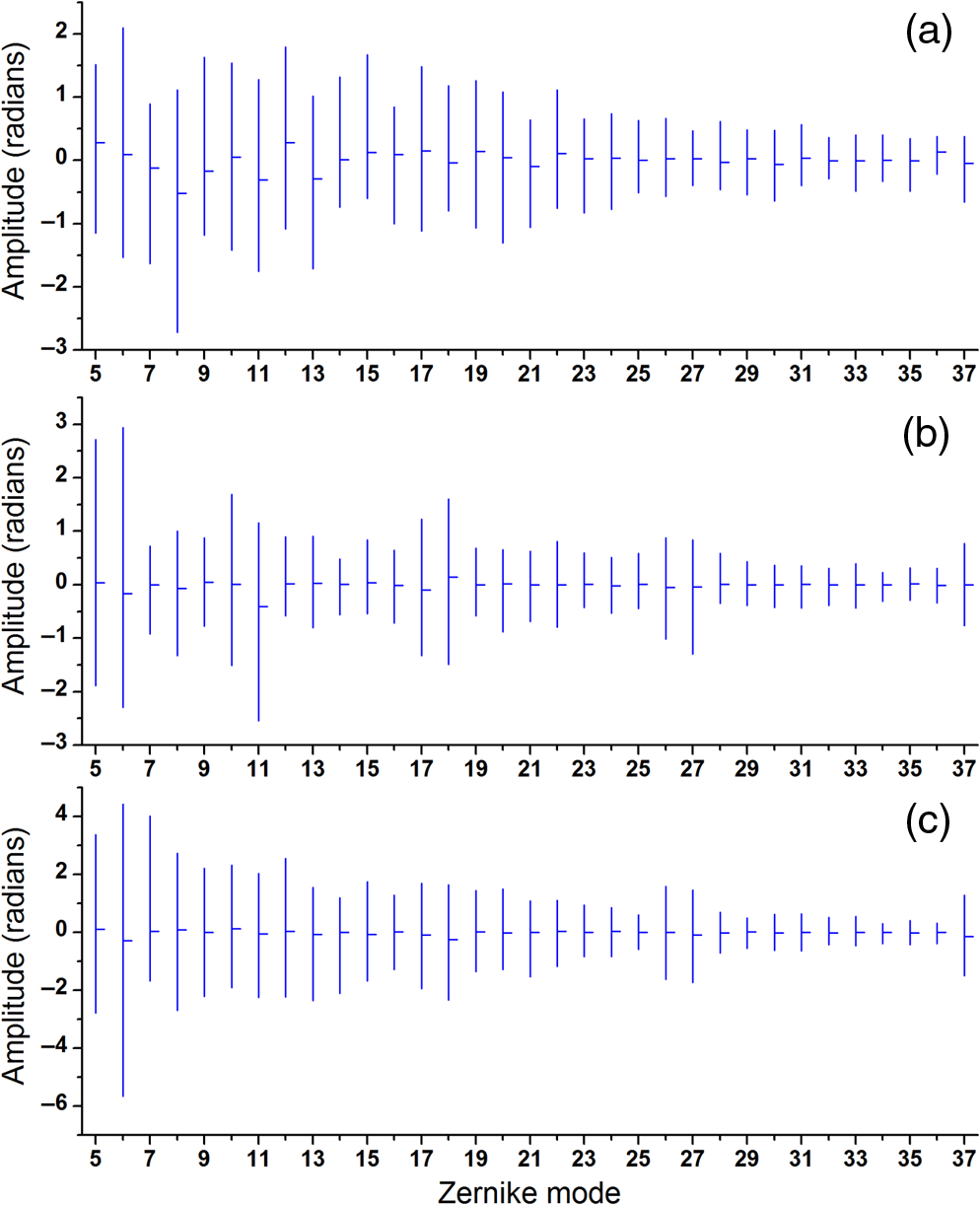

To practically maximize correction of the Zernike modes across the field of view in a scanning system, it is necessary for a deformable element to rapidly respond to the changing tissue aberrations. We therefore use the transition rate of the modes to estimate the additional residual wavefront error that occurs due to a lag in the frequencies of the correction element (such as a DM) behind the fast axis scanner and the gradient of Zernike modes in the sample. To assess the refresh rate of a desirable correction element, we calculate the gradient of modes in horizontal direction (the direction of the fast axis scan). We perform a 9-point first-order numerical derivative

Eq. (15)

$$\nabla {\phi }_i=[Z_i]\otimes \frac{[\frac{1}{280},-\frac{4}{105},\frac{1}{5},-\frac{4}{5},0,\frac{4}{5},-\frac{1}{5},\frac{4}{105},-\frac{1}{280}]}{2h},$$

where $h$ is the distance between two points on the image plane and brackets indicate the Zernike mode $i$ value across the horizontal axis in matrix form. Now, we can write an equation to estimate the wavefront error caused by stepping or pixelation of correction due to having less frequency of correction than signal collection, in the form

Eq. (16)

$${\sigma }_s=\sqrt{\sum _i{(⟨\nabla {\phi }_i⟩aN\frac{f_{\mathrm{s}}}{f_{\mathrm{c}}})}^2},$$

where $a$ is the pixel size, $N$ is the number of pixels horizontally, $f_{\mathrm{s}}$ is the scanning frequency, $f_{\mathrm{c}}$ is the frequency of the correction element, and the brackets indicate an average over the field of view. Where there is a significant difference between the frequencies of scanning and correction, the discrepancy between the sample aberrations modeled by Zernike modes 5 to 37 and the corrective elements on the scanner lead to an increase in the wavefront error. This error results in only a portion of the best-case theoretical correction (i.e., ${\sigma }_{\mathrm{res}}=1.25$, $\text{Strehl ratio}=20\%$) being achieved. When quantified by ${\sigma }_s$ as a function of correction frequency at a fixed laser scan rate [Fig. 10(a)], the additional absolute error approaches zero. Using the ${\sigma }_s$ values, we calculate the Strehl percentage⁵⁶ using $S_{\mathrm{scan}}=\exp (-{\sigma }_{\mathrm{s}}^2)$, assuming an 8-kHz resonant scanner and a 256 pixel width of the field of view [Fig. 10(a)], where 100% is full correction of Zernike modes 5 to 37. $S_{\text{scan}}$ therefore characterizes the reduction in Strehl ratio expected with inadequate scanning frequency.

Fig. 10

(a) Analysis of the absolute wavefront error ${\sigma }_{\mathrm{s}}$ caused by inadequate corrective element frequency response with a fixed 8-KHz beam scan and the commensurate improvement of the Strehl percentage ($S_{\text{scan}}$). These metrics indicate a faster corrective element approaches full compensation of Zernike modes 5 to 37 at each point in the raster scanned field of view. (b) Analysis of effectiveness of residual wavefront error correction given the number of elements on the correction device.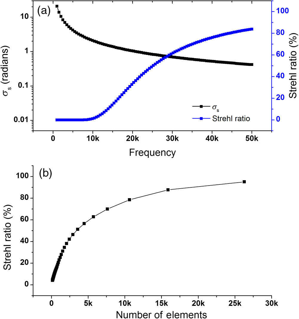

Having calculated the number of segments, it is important to know how much the size of each segment affects the wavefront correction. In other words, having larger elements would average wavefront errors over a larger region where a lot of variation exists due to smaller features of the sample. We therefore calculated the wavefront error by convolving the residual wavefront error with a uniformly distributed (and normalized—sum equals 1) kernel $K$ that mimics the segment size

Eq. (17)

$${\sigma }_{\mathrm{seg}}={\left\{\frac{{\iint }_A{[{\phi }_e(\mu ,\nu )-({\phi }_e(\mu ,\nu )\otimes K_l)]}^2\mathrm{d}\mu \mathrm{d}\nu }{{\iint }_A\mathrm{d}\mu \mathrm{d}\nu }\right\}}^{\frac{1}{2}},$$

where the subscript $l$ denotes different segment size. Figure 10(b) shows Strehl ratio versus the number of elements in the DM.

4.

Discussion

By characterizing the optical aberrations generated when performing SHG imaging, we are able to evaluate the degree of AO correction and to determine DMs, SLMs, or DMDs required to attain near-diffraction-limited imaging deep in the cranial bone. AO correction using these correction elements will allow us to image fine structures in the bone marrow (e.g., subcellular features, such as mitochondria) that would not be resolvable using a lower NA, lower magnification objective lens to reduce distortions;⁵⁷ or by moving to longer wavelength two-photon or three-photon excitation that requires an exotic optical assembly and fluorophores.⁶ Our bone characterization approach can also be used to directly estimate wavefront aberrations and be applied to a correction algorithm; however, it should be noted that the illumination wavelength used to estimate aberrations should match the wavelength to be corrected.

We found that many low-order optical aberrations produced by the bone marrow can be corrected with a DM. However, as shown in Table 1, a minimum of a 1.25 radian RMS wavefront error is anticipated to remain after correcting Zernike modes 5 to 37, which leads to a maximum possible Strehl ratio of 20%. Our results show that a microelectromechanical system (MEMS) DM with stroke of $1.5\mu \mathrm{m}$ can be used to compensate these errors, which can make a perfect match with the correction function.⁵⁸ Using a MEMS DM is especially helpful due to their fast response time ($<20\mu \mathrm{s}$), with a moderate number of elements (52 to 144).

One challenge here is to capture all the high-order aberrations. Our optical setup takes advantage of an objective lens with NA of 1.1, which produces a two-photon beam waist of 326 nm.⁵⁹ Given the field of view, our resolution produces enough sampling to capture many high-order aberrations. There are expected to be scattering features smaller than our resolution, but our efforts provide a useful initial estimation, and we approximately account for this scattering using Eq. (8).

To further improve the Strehl ratio and achieve near-diffraction-limited imaging in vivo, a method for correcting the residual wavefront error is needed. Our estimates indicate that more than 23,000 segments are required to effectively correct for the scattering aberrations and restore the PSF. An SLM with $512\times 512\text{pixels}$ can work in this situation. The increase in the intensity of the focal spot over the average speckle intensity before correction is proportional to the number of segments.^30,60 Focusing through turbid media can be fairly slow because of the SLM’s response time, the large number of segments to be controlled, and convergence time of the algorithm used.^32,60–64 The speed of wavefront shaping can be increased dramatically by using a DMD instead of an SLM. By using a DMD, the depth of phase modulation will be replaced by only on/off switching depending on which rays contribute to the focus;^30–32 however, DMDs are capable of much higher modulation speeds of over 32 kHz (TI—DLP7000). DMDs can be used for wavefront shaping by either using off-axis holograms⁶⁵ or binary modulation.³⁰

Evaluation of the rate of transition of aberrations across the field of view demonstrated that wavefront correction across a $320\mu \mathrm{m}\times 320\mu \mathrm{m}$ field of view with a typical 8-kHz resonant scanner at correction frequency of 50 kHz can achieve an improvement up to 80% of the maximum Strehl ratio of a system correcting for Zernike modes 5 to 37 (i.e., ${\sigma }_{\mathrm{res}}=1.25$, $\text{Strehl ratio}=20\%$). This is due to the gradient of the calculated tissue aberrations and lagging of the typically slower corrective element behind the fast scan. Therefore, a balance between acquisition speed and aberration correction should be sought to balance the demands of video rate scanning, field of view size, and the available speed of correction elements. Since residual aberrations that are not captured by Zernike modes 5 to 37 play a significant role in reducing the overall Strehl ratio, we suggest a combination of a DM and DMD to reduce most of the aberrations. In a system with both correctors working at a 20-kHz refresh rate and a line scanning frequency of 4 kHz, AO corrected two-photon imaging at the speed of 15 frames per second on a $320\mu \mathrm{m}\times 320\mu \mathrm{m}$ field of view or larger would be within reach.

5.

Conclusion

In conclusion, we calculated the wavefront phase deviations for focusing beams into the highly scattering cranial bone of a mouse, using a linear ray tracing method, and the refractive indices of the bone mapped from an image stack acquired using SHG of collagen. In the current model, bone cavities are treated as having a homogenous refractive index. By calculating the projection of points across the field of view to the back pupil plane, we calculated the projected wavefronts and extracted Zernike polynomials from them. We used the Zernike modes within the current limitations of typical DMs to produce a correction function. We found a minimum of 1.54 radians RMS wavefront error produced in Zernike modes 5 to 37. We further calculated the residual wavefront error, which showed a significant remaining RMSE of 1.25 radians, corresponding to a maximum of 20% Strehl ratio. Based on our calculation of the correlation length of the wavefront RMS error, we suggest that wavefront correction elements with a large number of segments ($>\mathrm{23,000}$) with frequencies of the correction elements and the resonant scanner in a proportion near unity must be used to effectively compensate for distortions produced by a highly scattering medium, such as bone, to restore a diffraction limited imaging system.

We show that the optical aberration measurements that are extracted from the SHG imaging of bone can be used as a priori information in an open-loop AO system or as the initial state in a closed-loop AO correction system to speed up the process. This information can be very helpful especially for the binary correction to enhance the convergence of the algorithm. In future work, we will extend our investigation to more fully characterize multilayered biological environments.