
|
|
1.IntroductionThe last several years have witnessed the development of numerous methods and techniques for obtaining two principal optical properties of tissue: the absorption coefficient () and transport (reduced) elastic scattering coefficient ().1–3 These parameters are used in the clinical context to: (1) diagnose pathological conditions or metabolic states and (2) monitor efficacy of therapeutic treatments. Optical absorption reflects the process of light attenuation by physiologically relevant chromophores, such as hemoglobin, melanin, carotenes, lipids, and water. Using a wavelength-dependent linear-square fit of absorption coefficient values and the Beer–Lambert law, the concentrations of individual chromophores can be calculated.4–7 Additionally, optical scattering by tissue reflects the probability of light being deflected by its structural components, such as interstitial water, cell membranes, nuclei, and other organelles, as well as structural fibers.8–11 Thus, macroscopic structural variation of tissue can be derived from scattering coefficients (amplitude and power) by Mie theory,12 characterized by an exponential monotone decrease, relative to wavelength. Hence, the separate measurement of absorption and scattering parameters as a function of wavelength can provide a comprehensive biochemical, morphological, and histochemical characterization of the tissues under study. This broad range of tissue parameters interrogated may be used to noninvasively diagnose disease even in very early stages. The range of optical methods applied to determine the optical properties of biological materials may be broadly divided into direct and indirect techniques. Direct methods rely directly on the experimental results, without any model of photon migration. Indirect methods are more complicated in their use, involve mathematical models and/or simulations of light propagation, and require sophisticated (and sometimes expensive) instrumentation.13–16 Time-resolved diffuse reflectance,17,18 frequency domain,19–21 spatially resolved continues wave,22–26 low coherence interferometry,27,28 and oblique incidence reflectometry29,30 are among the methods used to extract optical properties of sample tissue. Each of these methods has varying capabilities regarding accuracy, levels of noise and artifacts, field of view (FOV), spatial and temporal resolution, speed, penetration depth, etc. Among techniques recently developed for optical characterization of turbid media is spatially modulated illumination, known also as spatial frequency domain.31,32 With this technique, periodic illumination (sinusoidal grid) patterns are projected to separately map tissue absorption and reduce light scattering over a wide FOV, in a noncontact and scan-free fashion. The advantages of this imaging technique include capability of depth sectioning, as well as wide-field and wild-range imaging, ease of use, and relatively low cost due to its minimal number of optical elements. The technical capabilities of spatially modulated illumination have been well documented over the last 12 years, with successful demonstration in phantom, animal, and human studies.33–40 In the context of these contemporary techniques, this work aimed to apply structured illumination to acquire optical properties of tissue-simulating phantoms and human tissue in the near-infrared (NIR) region (600 to 1000 nm). As mentioned above, the application of spatially modulated illumination to quantify tissue properties was recently established in imaging setup and spectroscopy by several research groups. The innovation of the present study lies in the combination of both spectrometer and camera channels delivering simultaneous readings and in the ease of deriving optical properties. In this hybrid apparatus, the sinusoidal patterns are projected sequentially at low and high spatial frequencies (0 and , respectively), and the diffuse reflected light is recorded simultaneously by a single noncontact spectrometer and two separate CCD cameras. The system’s distinct advantage over other methods is that it allows each method of signal capture to complement gaps in the other’s capabilities, delivering clinically relevant information regarding tissue properties at high spatial and spectral resolution. This study builds on previous work advancing optical spectroscopy of tissue by sinusoidal patterns of spatially modulated light31 and, to the best of our knowledge, is the first to combine such an illumination setup with parallel recording by complementary spectrometer and camera array channels. The outline of the present paper is as follows: in Sec. 2, we provide details of the system operation, tissue property quantification analysis, and the calibration procedure to account for the system response. Section 3 will be devoted to experimental results measured from both phantoms and the human hand, as well as the calculation of tissue hemoglobin oxygen saturation. Additionally, we discuss the feasibility of reconstructing optical properties with recent analytical camera modeling.41 Finally, in Sec. 4, we discuss the results, future development, and the potential clinical and research applications of the technique. 2.Experimental Study2.1.Ethics StatementThe experiments involving humans in this work were approved by the Institutional Review Boards of Ariel University, and informed consent was obtained from all participants before measurements. 2.2.System DescriptionThe experimental system is drawn schematically in Fig. 1(a). The system integrates two channels: spectrometer and CCDs fed by the same sinusoidal fringe illumination. Optical measurement is configured as follows: sinusoidal patterns (fringes), generated in MATLAB® software, are serially projected onto the sample by a portable LED-based picoprojector (Aiptek, V10, LCoS Technology), passing through a collimated achromatic lens system (LS1). The collimated patterns are serially projected four times in total: three times at a fixed spatial frequency of , each time at different phases (0 deg, 120 deg, and 240 deg) to determine the reduced scattering coefficient, followed by a final illumination at zero spatial frequency () without any phase shift (planar unmodulated illumination) for determination of the absorption coefficient. Demonstration of reflection patterns at these frequencies is shown in Fig. 1(b). While higher spatial frequency patterns are primarily sensitive to scattering changes but insensitive to absorption, the lower spatial frequency patterns are far more sensitive to changes in absorption than are they to scattering.32,42,43 As illustrated, the diffusely reflected light is recorded simultaneously by both CCD cameras and the spectrometer, which view the same region through the beam splitters (BSs) in a noncontact fashion. In this way, the diffusely reflected light emanating from the sample is first split into two separate optical paths by BS1: the first propagate to a portable compact fiber-coupled spectrometer (USB4000-VIS-NIR, Ocean Optics) and the second propagate to BS2 where light is divided again before detection by two separate CCD cameras (Guppy PRO, F031B, Allied Vision Technology). Each camera, capable of imaging up to 123 frames per second at full resolution, produces a 14-bit monochrome image with pixel spatial resolution, at pixel size of . Each camera is equipped with a zoom lens system (Computar, 75 to 150 mm, f#/2.8, New York) and an optical bandpass filter (10-nm FWHM BPF, Thorlabs) of 650 nm (BP1) or 800 nm (BP2), respectively, placed in the front of the camera, enabling dual-band imaging. Thereby, the diffusely reflected light is first collected concomitantly by both channels and then filtered by each respective BPF prior to simultaneous image capture of the identical field. Camera exposure time and gain were manually adjusted for each wavelength filtering during the calibration process; both settings were found to be higher at 800 nm than at 650 nm because of the reduced quantum efficiency of the CCD at longer wavelengths. While originally obtained images were of high signal-to-noise ratio, collected diffuse images were nonetheless normalized prior to processing to decrease discrepancies in pixel intensity of the filtered images. The delivered light to the spectrometer from BS1 was filtered by adjusted pinholes and focused by a second lens system (LS2) onto a single optical fiber, (, ), coupled to a connection interface to the spectrometer, measuring at a spectral range of 400 to 1000 nm. The optical fiber, placed on the center of BS1 and LS2, is positioned by a metallic rod attached to an mechanical stage translation for position control to ensure maximum light collection. In contrast to the CCDs, the spectrometer recorded a range of wavelengths that dramatically increased the spectral resolution. However, the improved spectral resolution came at the expense of the field of vision imaged since single-point measurements cannot provide spatial information. The spectrometer interfaces to the computer via USB 2.0 port and is controlled by Ocean Optics software (OOI Base 32). Each set of data acquired by the spectrometer includes the measurements of replicate spectra () during a single data collection session. These spectra are later assembled together to a single average spectrum, thereby increasing the signal-to noise ratio by a factor of . The average time required to acquire one complete measurement was 10 s. The entire setup is controlled by MATLAB® software (MathWorks, Massachusetts) and imaging acquisition, synchronization, and data processing are achieved using in-house developed MATLAB® scripts on a laptop computer equipped with an Intel® Core™ -3210M processor running at 2.5 GHz with 4 GB memory. 2.3.Data AnalysisEach sample was illuminated at low () and high () spatial frequencies to determine the absorption and reduced scattering coefficients, respectively. Consequentially, measurements taken at these two extreme spatial frequencies resulted in contrasting sensitivities to absorption (low frequency) as well as reduced scattering (high frequency) coefficients.32,42,44 In this work, the derived values of optical properties and chromophore responses were considered to be average values resulting from sampling bulk volume. The remitted reflectance was captured simultaneously by the respective channels and saved for processing and analysis off-line using in-house scripts written in MATLAB®. Prior to camera image and spectrometer raw data analysis, the collected diffuse images at both wavelengths and raw vectors were normalized and filtered to reduce different sources of noise. 2.3.1.Camera processingFor the respective dataset of each repetition, each individual image is an average of 50 consecutive frames captured by the camera to maximize signal intensity, thereby optimizing signal-to-noise ratio. Thus, four averaged serial images were acquired simultaneously by each camera, one at low frequency (DC) and three phase shifted at high frequency (AC). Each experiment was performed in replicates of 10, resulting in 40 images (10 DCs and 30 ACs) per camera. For each DC image acquired at a specific wavelength, a region-of-interest (ROI) was selected manually by the investigators, and the mean value of this ROI, , was calculated using the mean2 function in MATLAB®. DC illumination was also projected upon a diffuse reflectance standard (white Spectralon, WS-1, Ocean Optics) in the FOV, and ROI and mean value , as previously, were obtained. The normalized reflectance was calculated by subtraction from dark response , and a natural logarithmic function () was obtained to derive the absorption coefficient by Dark response, , was characterized by acquiring an image while the light source was turned off, and it is related to the thermal noise of the CCD array. The white surface provides reflectance and was used to compensate for the spectral shape of the light emitted by the projector and the wavelength-dependent sensitivity of the detector and of the detecting system components. Following 10 repetitions (), 10 absorption values per wavelength () were created, , and then averaged to obtain a single mean value of absorption Once the absorption coefficient at different wavelengths is known and combined with the wavelength-dependent molar extinction coefficients , metabolic properties () such as perfusion, oxygenation, and chemical content (concentrations of hemoglobin, lipids, water, etc.) can be derived by applying the least-squares solution to the Beer–Lambert law, , as commonly employed in tissue optics.45 represents the number of chromophores in tissue. This equation shows the absorption coefficient () at a given wavelength () to be a linear combination of the extinction coefficients () and their corresponding chromophore concentrations ().High-spatial frequency reflectance at wavelength was recorded in three sequential images at differential 120 deg phase shifts, from which the reduced scattering coefficient image was approximated as follows: where , , and represent the captured reflectance images at spatial phases of 0 deg, 120 deg, and 240 deg, respectively. Similar to absorption, using this relation we mapped light scattering at each wavelength on a pixel level. From this scattering image, an ROI was selected and the mean value was calculated (mean2 in MATLAB®). Following 10 repetitions, a vector of 10 scattering coefficient values was created and then averaged to derive a single reduced scattering coefficient for each wavelength () Please note that by averaging scattering images at each wavelength, the scattering spectra of the sample can be derived via the wavelength-dependent power law function in the form of , where is the scattering amplitude and sp is the scattering power (slope).46,47 This functional dependence is supported by numerous studies and is commonly employed for tissue optics.48 By analyzing the spectra of scattered light, information regarding macroscopic cellular morphology can be retrieved through the scattering magnitude () and power (sp). In particular, sp is related to mean size of the tissue scattering agents (cell membrane, nuclei, lysosomes, mitochondria, and other organelles in the cytoplasm) and defines spectral behavior of the reduced scattering coefficient, while related to density and distribution of scattering agents, such that the value and sign of sp () is a frequently used tool for differential diagnosis of tissue pathologies.48–502.3.2.Spectrometer processingSignal processing by the spectrometer is similar to that outlined above, with a few modifications. Once the DC illumination is projected onto the sample, the remitted reflectance from the entire observed area is averaged by LS2, transmitted to the spectrometer through single fiber optic probe, and then recorded, creating a vector comprised of the values from hundreds of wavelengths. In contrast to that described above, Eq. (1) is carried out automatically by the spectrometer software, after which the log operation is performed off-line. Following 10 repetitions, 10 absorption spectra per repetition are recorded and then averaged together to obtain a single absorption spectra wherein , with a spectral resolution of . To eliminate the high-frequency noise produced by the spectrometer, absorption spectra were then filtered using a second-order Savitzky–Golay filter in MATLAB®. With the AC illumination, each spectra (, , and ) is saved as a vector: , , , and Eq. (3) is performed, creating a scattering coefficient vector over hundreds of wavelengths per repetition ()At the end of repetitions, 10 vectors of scattering coefficient values at multiple wavelengths are created and then averaged to derive a single vector of the reduced scattering coefficient In contrast with the image processing algorithm, the spectral resolution of the scattering spectra dramatically increases, enabling the derivation of tissue structural variations (, sp) via the power law equation ().It should be stressed that to reduce data acquisition time, thereby allowing rapid extraction of optical properties and speeding up the imaging procedure, the current setup can project only the three AC frames and obtain the DC () image by the following calculation: given that the DC image is proportional to the absorption coefficient [through the log function, Eq. (1)]. Please note that in the original setup (Ref. 31) a total of six images per wavelength are needed (three phases each for AC and DC) to extract sample optical properties. Recent works aimed toward development of real-time optical imaging based on structured illumination have reported single51,52 or coupled projection53 images per wavelength. Comparison of the DC image obtained by Eq. (8) with uniform DC illumination on a human hand at 800 nm (Fig. 2) demonstrates good agreement between the two approaches. Also shown in the same figure is the absorption spectrum obtained by Eq. (8) relative to the planar (uniform) illumination. Spectra appear identical, with maximum difference amounting to less than 0.5% (at 990 nm) as presented by the difference plot shown in the same figure. Hence, it may be feasible to extract the absorption spectra or coefficient with Eq. (8), in turn reducing the acquisition and processing time. Nevertheless, since in the current study we were not concerned with real-time imaging, we used the four-projection method.Fig. 2(a) AC frequency () with phase shift of 120 deg between patterns. (b) DC frequency obtained by Eq. (8). (c) Direct DC (planar or uniform) illumination. (d) Difference image highlights zero discrepancies between the two. (e) Absorption spectrum comparison obtained by Eq. (8) against the DC illumination. The bottom graph marked with the dash-dot line represents the difference between absorption spectrum plots.  2.4.CalibrationA calibration procedure was utilized prior to data acquisition to reduce errors in the measurement of optical properties potentially resulting from the approximations made in Eqs. (1) and (3), due to possible system variabilities stemming from projector source fluctuations and nonlinearity, or from variations in the collection efficiencies of the camera and spectrometer. The calibration process made use of tissue phantoms as a reference standard. These phantoms were constructed from intralipid and dyes as described in detail previously,54 and their optical properties over the wavelength range of 650 to 1000 nm were measured using the oblique-incidence reflectometry method.55 The obtained spectral absorption and reduced scattering graphs were found to be similar to those determined by the two-distance steady state frequency domain photon migration system used in Ref. 54. In our work, phantoms aid us in determining two scale factors, and , as respective estimators of the true scattering and absorption coefficients, respectively. Each of these spectral factors was determined as the ratio between estimated experimental values to the actual reference values. Once determined, these ratios were applied later to divide Eqs. (2), (4) and (5), (7) for future validation of unknown sample optical properties. The value of each factor was determined according to the average across two calibration experiments taken from two separately measured phantoms. Experimentally, we found that the camera scale factor deviated from those of the spectrometer. After and were determined, the validation process continued with the measurement of a new phantom with known optical properties. We then applied the same process in a second set of experiments on normal human skin tissue. 3.Results and DiscussionAs mentioned above, calibration and validation experiments were conducted with two different solid-tissue phantoms with known optical properties over the wavelength range of 650 to 1000 nm. In total, a set of two phantoms for calibration and two phantoms for validation purposes was used. Following the calibration process, a scale factor was determined for the respective true values of scattering and absorption coefficients. These factors were used later for estimation of the true optical properties of the validation phantoms and of the human tissue. Representative traces reconstructing the absorption and reduced scattering coefficients at 650 nm (left column) and 800 nm (right column) for validation phantom #1 through camera processing over 10 repetitions during nonconsecutive days () appear in Fig. 3(a). The data points in the graphs represent the mean and the error bars refer to the standard error calculated for the measurements. The error bars for the scattering are not seen because of minute deviation from the mean. A similar trend and average values were observed for validation phantom #2 (data not shown). Stability of the measurements between days of experimentation indicates the minimal influence of artifacts on measurements. The results for the same phantom derived by spectrometer processing at the two specific wavelengths are presented in Fig. 3(b). Also here, the error bars for the scattering are not seen, and overall stability in measurements is observed. The extracted average values from both figures are given in Table 1. A difference in both estimated coefficients between the camera and the spectrometer channels is recognizable, particularly for the scattering coefficient, with a difference between the two methods at 650 nm. By contrast, less than 5% difference in absorption value between the two channels was found. Figure 4 presents bar graphs summarizing the average and standard error of both extracted optical properties at the two wavelengths as obtained by the camera and the spectrometer channels for validation phantoms, in comparison with their anticipated values. Both figures clearly demonstrate discrepancies between the calculated optical properties and their actual values. Fig. 3(a) Representative profiles of the absorption (upper panels) and reduced scattering coefficients (lower panels) at two wavelengths during validation on tissue-mimicking phantom (not included in the calibration process) using the camera channel. represents the mean over four nonconsecutive days. Data points represent the mean, and a bar refers to standard error. Error bars for the scattering are not seen because of minute deviation from the mean. (b) The same as in (a) but reflecting the spectrometer channel.  Table 1Comparison of recovered average optical properties ± standard error (SE) for absorption and reduced scattering coefficients of phantom #1 between CCD cameras channel and spectrometer channel as extracted from Fig. 3. ± is the root of the sum of the error squares; ∑i=110(SE)i2.
Fig. 4Quantification of (a) the absorption and (b) scattering coefficients at the two wavelengths obtained by the camera and spectrometer channels following validation analysis of validation phantom in comparison with the actual value. Each bar represents the over ten repetitions during four nonconsecutive days.  Referring to Fig. 4(a), the difference at both wavelengths between the extracted absorption coefficient and their anticipated values for both channels reached 20%, with interchannel deviation of . For the reduced scattering coefficient, Fig. 4(b), an average deviation of from the actual values was observed by the camera array, while variance of and was detected among the spectrometer measurements at wavelengths 650 and 800 nm. Differences between detected and actual values may have several origins: (1) differential geometry employed by the two channels for reflected light collection, (2) aberrations in light collection efficiency, (3) the different methods by which the FOV is selected: with the camera an ROI is selected manually while with the spectrometer the entire FOV is averaged into one single value, unavoidably introducing additional noise, and (4) approximation of the optical properties calculated using Eqs. (1) and (3). Other sources of error and their possible solutions were reported recently.56 We believe that such discrepancies can be minimized and that better precision can be obtained in the future by utilizing a larger set of phantoms possessing different optical properties over the spectral band in which the measurements were taken (650 to 1000 nm) to optimize calibration factors. Procedures for correction of sample height- and angle- (surface profile) based structured illumination, suggested previously to recover optical properties more accurately,52,57,58 will be applied in our ongoing research. Next, the system was used to measure the optical properties and hemoglobin oxygen saturation of skin tissue of two healthy adult volunteers. Measurements were obtained from the right back hand of subject D (male) and the left back hand of subject M (female); in both subjects, the observed area was the back wrist adjoining the base of the hand. Figure 5(a) shows a photograph of the region captured from subject D, and under DC [Fig. 5(b)] or AC illumination [Fig. 5(c)], alongside plots of the corresponding measured absorption and scattering spectra by the spectrometer [Fig. 5(d)]. A clear decrease in absorption spectrum is evident in the upper panel of Fig. 5(d), which we attribute to differences in concentration of both hemoglobin and melanin. At the same time, two peaks at and 980 nm were observed, corresponding to lipid and water absorption, respectively.59,60 By fitting the skin’s reduced scattering spectra to a scattering power law (), we show monotonous spectra decrease, correlating with increased wavelength, such that (scatter density) and (scatter average size). The sp result is within the range documented by other groups (Table 1 in Ref. 61). As commonly reported, between 700 and 900 nm, absorption by skin chromophores is minimal, while scattering effects are dominant,62–64 as reported presently. The bar graphs shown in Fig. 6 summarize the average and standard error of both optical properties from the two volunteers (subjects D and M) at the two wavelengths recorded by the camera (upper panel) and spectrometer (lower panel), relative to reference values and values obtained through the diffusion model theory [Eq. (9)]. As expected, the optical properties differ between volunteers as a result of their different BMIs and skin color. As in the phantom experiments, discrepancies were detected between the calculated and reference values: all obtained parameters were lower than reference values, with the exception of scattering at 800 nm in the CCD channel. A possible explanation for these differences may lie in the reference values being averaged from five published studies using different experimental conditions, model samples (skin color, age, etc.), and measuring setup.63–68 Additionally, partial volume effects may contribute to this discrepancy. Another point that should be taken into account in future experiments with human subjects is the correction of absorption against water concentration in addition to correction sample profile (height and angle mentioned above), which can lead to strong variations in optical properties.69,70 Fig. 5(a) Photograph of the right back hand of subject D. Two spatial frequencies that were sequentially projected: (b) DC and (c) AC illumination, respectively. (d) Plots of the measured absorption (upper panel) and reduced scattering spectra (lower panel) from 650 to 1000 nm through the spectrometer processing channel. As expected, the scattering coefficient follows a power law dependence seen in tissue.  Fig. 6Statistical analysis of the optical properties from two volunteers (subject D and subject M) at the two wavelengths obtained by (a) the camera and (b) spectrometer channels. Comparison of literature-reported values and the model theory [Eq. (9)] are illustrated. Subject D: gender: male, age: 21 years old, BMI: 16.90 (underweight), hand color: black, hand side: right back wrist area. Subject M: gender: female, age: 25 years old, BMI: 27.34 (overweight), hand color: white, hand side: left back wrist area.  In addition, a comparison with the results obtained using recent light propagation models was performed and plotted in Fig. 6. With this model, the total diffuse reflectance measured from a semi-infinite medium using an exponentially decaying source is given as41 where is the diffuse reflectance at the surface and is a dimensionless parameter that takes into account the incident power, numerical aperture of the lens camera, and refractive index difference (air ↔ medium). The absorption coefficient is represented by , is the boundary coefficient that accounts for differences in refractive indices, and is the total interaction coefficient (sum of the absorption and reduced scattering coefficients). Sometimes is also referred to as the reduced extinction coefficient or transport coefficient. The diffusion coefficient, , is directly related to the optical properties by the following equation: . We used a tissue-like phantom with known optical properties over the NIR range to determine the values of and through measured diffuse reflectance. The factors and were obtained by minimizing the least square between the measured and theoretical [Eq. (9)] diffuse reflectance values by the Levenberg–Marquardt algorithm in MATLAB® for a given set of optical properties, which yielded and . Once Eq. (9) is calibrated against the experimental reflectance, it can be applied in an inverse manner to recover tissue optical coefficients (absorption and reduced scattering). When comparing our measurements, differences are evident, which may be explained by the approximations used in Eq. (9) (see Ref. 41) and in our equations [Eqs. (1) and (3)] and by the use of only one phantom to derive the and factors during the calibration procedure. Therefore, error may be minimized in the future by use of larger sets of phantoms and statistical analyses to derive optimal values for and . Thus, extending the calibration range is one of the subjects of our continued efforts to develop a more accurate and reliable system for derivation of optical properties of tissue.Following the extraction of tissue optical properties, we continued with an estimation of hemoglobin oxygen saturation level (). Quantitative assessment of human hemoglobin oxygenation levels is an important tool for monitoring tissue health and for managing a variety of clinical situations. There are several approaches currently in use for evaluating oxygen saturation by tissue spectroscopy. Among them is that defined by the following:71 where and are the known molar extinction coefficients of oxyhemoglobin () and deoxyhemoglobin (Hbr), respectively, with the constant wavelength values of and . Based on our measurements, introducing the recovered absorption coefficients into the above equation yielded the oxygenation saturation levels reported in Fig. 7. The percent variance in saturation levels between channels for each subject demonstrate less than full agreement between channels (less than 30%). Discrepancies between individuals (less than 20%) may be explained by different skin color, age, gender, motion artifacts, etc. Furthermore, since a large area is sampled by the system, regional heterogeneity of tissue as well as the volume effect (sampling different layers including epidermis, dermis, subcutaneous layer) can highly influence the measured absorption values and hence the oxygen saturation level. Moreover, the calibration process was performed on a homogeneous, flat monolayer medium, while human skin, in contrast, is comprised of highly heterogeneous layers. Furthermore, the presence of additional chromophores, such as melanin found in living tissue, may introduce error to the calculation of oxygen saturation by Eq. (10). Nevertheless, the oxygen saturation values obtained by both channels are in good agreement with the average range of tissue saturation reported elsewhere.72–74Fig. 7Comparison of tissue oxygenation saturation level between volunteers and between channels. The percent change for each possibility is given. 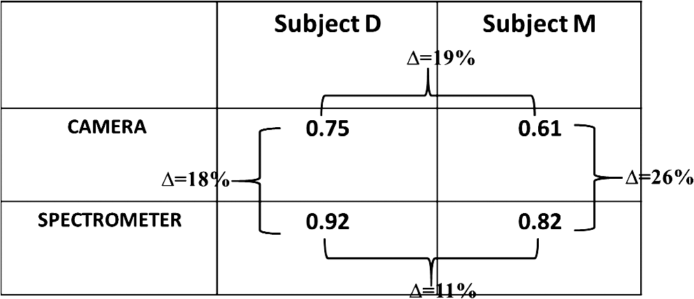 Hemoglobin oxygen saturation levels can also be derived from the intensity of reflected light; since the wavelength of 800 nm is close to the isosbestic point where oxy- and deoxyhemoglobin absorbs light equally, total hemoglobin concentration (THC) can be readily obtained. In contrast, at 650 nm, the overwhelming majority of absorption is attributed to deoxyhemoglobin (Hbr). Hence, by analyzing the spatiotemporal changes in diffuse reflected light at 650 and 800 nm, the variations in hemoglobin oxygenation may be derived. Since , saturation level can be calculated by A representative spatial image and its histogram distribution derived using this equation for subject M is presented in Fig. 8. Scale values of oxygen saturation are represented by the scale down the image. Averaging the values of the image map revealed , amounting to a 9% deviation from that obtained with Eq. (10) (Fig. 7, upper-right). Fig. 8(a) Photograph of the left hand of subject M with the dashed rectangle highlighting the selected ROI selected during processing. An example of the absorption and scattering spatial maps at 650 nm within the selected ROI is also presented. (b) Tissue oxygen saturation map of the ROI with a corresponding histogram (c) was generated by Eq. (11). This mapping reveals spatial oxygen saturation heterogeneities within the measured tissue. The horizontal color bar represents the saturation value of each pixel in the map, such that higher saturation values correspond to brighter pixels. Conversion of the saturation map into histogram distributions demonstrated localized changes in the saturation levels at single-pixel resolution and illustrates the distribution of oxygen saturation within the FOV. The vertical axis in the histogram reflects the number of counts in each bin, and the solid curve is a Gaussian fit with mean and standard deviation of 0.70 and 0.062, respectively. Both map and histogram illustrate the fine resolution at which the system can image tissue oxygen saturation parameters.  4.SummaryIn this study, a noncontact optical setup integrating spectrometer and camera arrays was established to quantify optical properties of both tissue-phantoms and biological tissue over a large FOV by spatial light modulation (structured illumination). In this setup, sinusoidal light patterns are serially projected onto the sample at both low and high spatial frequencies to isolate the target’s absorption (linked to tissue metabolism) and scattering (related to tissue structure) properties. The diffuse reflected light is simultaneously acquired by single spectrometer and passes through two parallel narrow bandpass filters, each leading to an acquisition camera. In addition to the extraction of the tissue’s optical properties, we calculated hemoglobin oxygen saturation levels from the hands of two healthy volunteers (Fig. 7). A major advantage of this parallel optical configuration lies in the ability of each component to complement the other, enabling high spectral and spatial resolution. Since this combined platform provides complementary information both spectrally and spatially, it was able to detect variance between the optical properties recorded by the camera and spectrometer channels, as well as between the recovered absorption and scattering coefficients and those expected (Fig. 6). An additional validation methodology based on the theoretical model-based diffusion equation further revealed discrepancies between the calculated and theoretical values. The discussion raised several factors that may account for such differences, together with proposed adjustments to mitigate these potential artifact sources, as part of our ongoing research. We are currently optimizing strategies to further improve the system’s performance. The present work is not the first to demonstrate wide-band tissue optical spectroscopy utilizing sinusoidal patterns of spatially modulated light.75 However, to the best of our knowledge, there is no example of such combined spatially modulated optical setup for tissue optical characterization. ReferencesL. V. Wang and H.-I. Wu, Biomedical Optics: Principles and Imaging, Wiley, Hoboken, New Jersey
(2007). Google Scholar
J. G. Fujimoto and D. Farkas, Biomedical Optical Imaging, Oxford University Press, Oxford, England, United Kingdom
(2009). Google Scholar
D. A. Boas, C. Pitris and N. Ramanujam, Handbook of Biomedical Optics, CRC, Boca Raton, Florida
(2011). Google Scholar
W. G. Zijlstra, A. Buursma and O. W. Van Assendelft, Visible and Near Infrared Absorption Spectra of Human and Animal Haemoglobin, VSP Publishing, Utrecht, The Netherlands
(2000). Google Scholar
A. Sassaroli and S. Fantini,
“Comment on the modified Beer-Lambert law for scattering media,”
Phys. Med. Biol., 49
(14), N255
–N257
(2004). http://dx.doi.org/10.1088/0031-9155/49/14/N07 PHMBA7 0031-9155 Google Scholar
H. Z. Yeganeh et al.,
“Broadband continuous-wave technique to measure baseline values and changes in the tissue chromophore concentrations,”
Biomed. Opt. Express, 3
(11), 2761
–2770
(2012). http://dx.doi.org/10.1364/BOE.3.002761 BOEICL 2156-7085 Google Scholar
D. T. Delpy et al.,
“Estimation of optical pathlength through tissue from direct time of flight measurement,”
Phys. Med. Biol., 33
(12), 1433
–1442
(1988). http://dx.doi.org/10.1088/0031-9155/33/12/008 PHMBA7 0031-9155 Google Scholar
A. Cerussi et al.,
“In vivo absorption, scattering, and physiologic properties of 58 malignant breast tumors determined by broadband diffuse optical spectroscopy,”
J. Biomed. Opt., 11
(4), 044005
(2006). http://dx.doi.org/10.1117/1.2337546 JBOPFO 1083-3668 Google Scholar
D. Yohan et al.,
“Quantitative monitoring of radiation induced skin toxicities in nude mice using optical biomarkers measured from diffuse optical reflectance spectroscopy,”
Biomed. Opt. Express, 5
(5), 1309
–1320
(2014). http://dx.doi.org/10.1364/BOE.5.001309 BOEICL 2156-7085 Google Scholar
J. R. Mourant et al.,
“Mechanisms of light scattering from biological cells relevant to noninvasive optical-tissue diagnostics,”
Appl. Opt., 37
(16), 3586
–3593
(1998). http://dx.doi.org/10.1364/AO.37.003586 APOPAI 0003-6935 Google Scholar
M. R. Hajihashemi, X. Li and H. Jiang,
“Morphological characterization of cells in concentrated suspensions using multispectral diffuse optical tomography,”
Opt. Commun., 285
(21–22), 4632
–4637
(2012). http://dx.doi.org/10.1016/j.optcom.2012.07.043 OPCOB8 0030-4018 Google Scholar
V. V. Tuchin, Tissue Optics: Light Scattering Methods and Instruments for Medical Diagnosis, 2nd ed.SPIE, Bellingham, Washington
(2007). Google Scholar
B. C. Wilson, M. S. Patterson and S. T. Flock,
“Indirect versus direct techniques for the measurement of the optical properties of tissues,”
Photochem. Photobiol., 46
(5), 601
–608
(1987). http://dx.doi.org/10.1111/php.1987.46.issue-5 PHCBAP 0031-8655 Google Scholar
W. Cheong, S. A. Prahl and A. J. Welch,
“A review of the optical properties of biological tissues,”
IEEE J. Quantum Electron., 26
(12), 2166
–2185
(1990). http://dx.doi.org/10.1109/3.64354 IEJQA7 0018-9197 Google Scholar
M. S. Patterson, B. C. Wilson and D. R. Wyman,
“The propagation of optical radiation in tissue. II: Optical properties of tissues and resulting fluence distributions,”
Lasers Med. Sci., 6
(4), 379
–390
(1991). http://dx.doi.org/10.1007/BF02042460 Google Scholar
J. Falconet et al.,
“Estimation of optical properties of turbid media: experimental comparison of spatially and temporally resolved reflectance methods,”
Appl. Opt., 47
(11), 1734
–1739
(2008). http://dx.doi.org/10.1364/AO.47.001734 APOPAI 0003-6935 Google Scholar
S. Andersson-Engels et al.,
“Multispectral tissue characterization with time resolved detection of diffusely scattered white light,”
Opt. Lett., 18
(20), 1697
–1699
(1993). http://dx.doi.org/10.1364/OL.18.001697 OPLEDP 0146-9592 Google Scholar
T. Svensson et al.,
“Characterization of normal breast tissue heterogeneity using time-resolved near-infrared spectroscopy,”
Phys. Med. Biol., 50
(11), 2559
–2571
(2005). http://dx.doi.org/10.1088/0031-9155/50/11/008 PHMBA7 0031-9155 Google Scholar
S. Fantini et al.,
“Frequency-domain multichannel optical detector for noninvasive tissue spectroscopy and oximetry,”
Opt. Eng., 34
(1), 32
–42
(1995). http://dx.doi.org/10.1117/12.183988 Google Scholar
M. S. Patterson et al.,
“Frequency-domain reflectance for the determination of the scattering and absorption properties of tissue,”
Appl. Opt., 30
(31), 4474
–4476
(1991). http://dx.doi.org/10.1364/AO.30.004474 APOPAI 0003-6935 Google Scholar
B. J. Tromberg et al.,
“Noninvasive in vivo characterization of breast tumors using photon migration spectroscopy,”
Neoplasia, 2
(1/2), 26
–40
(2000). http://dx.doi.org/10.1038/sj.neo.7900082 Google Scholar
T. J. Farrell, M. S. Patterson and B. Wilson,
“A diffusion theory model of spatially resolved, steady-state diffuse reflectance for the noninvasive determination of tissue optical properties in vivo,”
Med. Phys., 19
(4), 879
–888
(1992). http://dx.doi.org/10.1118/1.596777 MPHYA6 0094-2405 Google Scholar
G. Zonios et al.,
“Diffuse reflectance spectroscopy of human adenomatous colon polyps in vivo,”
Appl. Opt., 38
(31), 6628
–6637
(1999). http://dx.doi.org/10.1364/AO.38.006628 APOPAI 0003-6935 Google Scholar
J. S. Dam et al.,
“Fiber-optic probe for noninvasive real-time determination of tissue optical properties at multiple wavelengths,”
Appl. Opt., 40
(7), 1155
–1164
(2001). http://dx.doi.org/10.1364/AO.40.001155 APOPAI 0003-6935 Google Scholar
H. Cen and R. Lu,
“Optimization of the hyperspectral imaging-based spatially-resolved system for measuring the optical properties of biological materials,”
Opt. Express, 18
(16), 17412
–17432
(2010). http://dx.doi.org/10.1364/OE.18.017412 OPEXFF 1094-4087 Google Scholar
R. Watté et al.,
“Metamodeling approach for efficient estimation of optical properties of turbid media from spatially resolved diffuse reflectance measurements,”
Opt. Exp., 21
(26), 32630
–32642
(2013). http://dx.doi.org/10.1364/OE.21.032630 OPEXFF 1094-4087 Google Scholar
Y. Zhao et al.,
“Deep imaging of absorption and scattering features by multispectral multiple scattering low coherence interferometry,”
Biomed. Op. Exp., 7
(10), 3916
–3926
(2016). http://dx.doi.org/10.1364/BOE.7.003916 BOEICL 2156-7085 Google Scholar
N. Dragostinoff et al.,
“Time course and topographic distribution of ocular fundus pulsation measured by low-coherence tissue interferometry,”
J. Biomed. Opt., 18
(12), 121502
(2013). http://dx.doi.org/10.1117/1.JBO.18.12.121502 JBOPFO 1083-3668 Google Scholar
G. Marquez and L. V. Wang,
“White light oblique incidence reflectometer for measuring absorption and reduced scattering spectra of tissue-like turbid media,”
Opt. Exp., 1
(13), 454
–460
(1997). http://dx.doi.org/10.1364/OE.1.000454 OPEXFF 1094-4087 Google Scholar
R. A. Wall and J. K. Barton,
“Oblique incidence reflectometry: optical models and measurements using a side-viewing gradient index lens-based endoscopic imaging system,”
J. Biomed. Opt., 19
(6), 067002
(2014). http://dx.doi.org/10.1117/1.JBO.19.6.067002 JBOPFO 1083-3668 Google Scholar
D. J. Cuccia et al.,
“Modulated imaging: quantitative analysis and tomography of turbid media in the spatial-frequency domain,”
Opt. Lett., 30
(11), 1354
–1356
(2005). http://dx.doi.org/10.1364/OL.30.001354 OPLEDP 0146-9592 Google Scholar
D. J. Cuccia et al.,
“Quantitation and mapping of tissue optical properties using modulated imaging,”
J. Biomed. Opt., 14
(2), 024012
(2009). http://dx.doi.org/10.1117/1.3088140 JBOPFO 1083-3668 Google Scholar
D. Abookasis et al.,
“Imaging cortical absorption, scattering, and hemodynamic response during ischemic stroke using spatially modulated near-infrared illumination,”
J. Biomed. Opt., 14
(2), 024033
(2009). http://dx.doi.org/10.1117/1.3116709 JBOPFO 1083-3668 Google Scholar
J. R. Weber et al.,
“Multispectral imaging of tissue absorption and scattering using spatial frequency domain imaging and a computed-tomography imaging spectrometer,”
J. Biomed. Opt., 16
(1), 011015
(2011). http://dx.doi.org/10.1117/1.3528628 JBOPFO 1083-3668 Google Scholar
A. J. Lin et al.,
“Spatial frequency domain Imaging of intrinsic optical property contrast in a mouse model of Alzheimer’s disease,”
Ann. Biomed. Eng., 39
(4), 1349
–1357
(2011). http://dx.doi.org/10.1007/s10439-011-0269-6 ABMECF 0090-6964 Google Scholar
S. Gioux et al.,
“First-in-human pilot study of a spatial frequency domain oxygenation imaging system,”
J. Biomed. Opt., 16
(8), 086015
(2011). http://dx.doi.org/10.1117/1.3614566 JBOPFO 1083-3668 Google Scholar
M. Laughney et al.,
“System analysis of spatial frequency domain imaging for quantitative mapping of surgically resected breast tissues,”
J. Biomed. Opt., 18
(3), 036012
(2013). http://dx.doi.org/10.1117/1.JBO.18.3.036012 JBOPFO 1083-3668 Google Scholar
R. P. Singh-Moon et al.,
“Spatial mapping of drug delivery to brain tissue using hyperspectral spatial frequency-domain imaging,”
J. Biomed. Opt., 19
(9), 096003
(2014). http://dx.doi.org/10.1117/1.JBO.19.9.096003 JBOPFO 1083-3668 Google Scholar
D. J. Rohrbach et al.,
“Characterization of nonmelanoma skin cancer for light therapy using spatial frequency domain imaging,”
Biomed. Opt. Express, 6
(5), 1761
–1766
(2015). http://dx.doi.org/10.1364/BOE.6.001761 BOEICL 2156-7085 Google Scholar
S. Nandy et al.,
“Characterizing optical properties and spatial heterogeneity of human ovarian tissue using spatial frequency domain imaging,”
J. Biomed. Opt., 21
(10), 101402
(2016). http://dx.doi.org/10.1117/1.JBO.21.10.101402 JBOPFO 1083-3668 Google Scholar
P. Symvoulidis et al.,
“Steady-state total diffuse reflectance with an exponential decaying source,”
Opt. Lett., 39
(13), 3919
–3922
(2014). http://dx.doi.org/10.1364/OL.39.003919 OPLEDP 0146-9592 Google Scholar
T. D. O’sullivan et al.,
“Diffuse optical imaging using spatially and temporally modulated light,”
J. Biomed. Opt., 17
(7), 071311
(2012). http://dx.doi.org/10.1117/1.JBO.17.7.071311 JBOPFO 1083-3668 Google Scholar
S. C. Kanick et al.,
“Sub-diffusive scattering parameter maps recovered using wide-field high-frequency structured light imaging,”
Biomed. Opt. Express, 5
(10), 3376
–3390
(2014). http://dx.doi.org/10.1364/BOE.5.003376 BOEICL 2156-7085 Google Scholar
D. Abookasis, B. Volkov and M. S. Mathews,
“Closed head injury-induced changes in brain pathophysiology assessed with near-infrared structured illumination in a mouse model,”
J. Biomed. Opt., 18
(11), 116007
(2013). http://dx.doi.org/10.1117/1.JBO.18.11.116007 JBOPFO 1083-3668 Google Scholar
T. H Pham et al.,
“Quantifying the optical properties and chromophore concentrations of turbid media by chemometric analysis of hyperspectral diffuse reflectance data collected using a Fourier interferometric imaging system,”
Appl. Spect., 55
(8), 1035
–1045
(2001). http://dx.doi.org/10.1366/0003702011952938 Google Scholar
J. R. Mourant et al.,
“Predictions and measurements of scattering and absorption over broad wavelength ranges in tissue phantoms,”
Appl. Opt., 36
(4), 949
–957
(1997). http://dx.doi.org/10.1364/AO.36.000949 APOPAI 0003-6935 Google Scholar
R. Graaff et al.,
“Reduced light-scattering properties for mixtures of spherical particles: a simple approximation derived from Mie calculations,”
Appl. Opt., 31
(10), 1370
–1376
(1992). http://dx.doi.org/10.1364/AO.31.001370 APOPAI 0003-6935 Google Scholar
V. V. Tuchin, Handbook of Optical Biomedical Diagnostics, SPIE Press, Bellingham, Washington
(2002). Google Scholar
X. Wang et al.,
“Approximation of Mie scattering parameters in near-infrared tomography of normal breast tissue in vivo,”
J. Biomed. Opt., 10
(5), 051704
(2005). http://dx.doi.org/10.1117/1.2098607 JBOPFO 1083-3668 Google Scholar
G. Zonios and A. Dimou,
“Light scattering spectroscopy of human skin in vivo,”
Opt. Express, 17
(3), 1256
–1267
(2009). http://dx.doi.org/10.1364/OE.17.001256 OPEXFF 1094-4087 Google Scholar
J. Vervandier and S. Gioux,
“Single snapshot imaging of optical properties,”
Biomed. Opt. Exp., 4
(12), 2938
–2944
(2013). http://dx.doi.org/10.1364/BOE.4.002938 BOEICL 2156-7085 Google Scholar
M. van de Giessen, J. P. Angelo and S. Gioux,
“Real-time, profile-corrected single snapshot imaging of optical properties,”
Biomed. Opt. Exp., 6
(10), 4051
–4062
(2015). http://dx.doi.org/10.1364/BOE.6.004051 BOEICL 2156-7085 Google Scholar
K. P. Nadeau, A. J. Durkin and B. J. Tromberg,
“Advanced demodulation technique for the extraction of tissue optical properties and structural orientation contrast in the spatial frequency domain,”
J. Biomed. Opt., 19
(5), 056013
(2014). http://dx.doi.org/10.1117/1.JBO.19.5.056013 JBOPFO 1083-3668 Google Scholar
F. Ayers et al.,
“Fabrication and characterization of silicone-based tissue phantoms with tunable optical properties in the visible and near infrared domain,”
Proc. SPIE, 6870 687007
(2008). http://dx.doi.org/10.1117/12.764969 PSISDG 0277-786X Google Scholar
J. Xia et al.,
“Monitoring sarcomere structure changes in whole muscle using diffuse light reflectance,”
J. Biomed. Opt., 11
(4), 040504
(2006). http://dx.doi.org/10.1117/1.2234278 JBOPFO 1083-3668 Google Scholar
N. Bodenschatz et al.,
“Sources of errors in spatial frequency domain imaging of scattering media,”
J. Biomed. Opt., 19
(7), 071405
(2014). http://dx.doi.org/10.1117/1.JBO.19.7.071405 JBOPFO 1083-3668 Google Scholar
S. Gioux et al.,
“Three-dimensional surface profile intensity correction for spatially-modulated imaging,”
J. Biomed. Opt., 14
(3), 034045
(2009). http://dx.doi.org/10.1117/1.3156840 Google Scholar
Y. Zhao et al.,
“Angle correction for small animal tumor imaging with spatial frequency domain imaging (SFDI),”
Biomed. Opt. Express, 7
(6), 2373
–2384
(2016). http://dx.doi.org/10.1364/BOE.7.002373 BOEICL 2156-7085 Google Scholar
T. Lister, P. A. Wright and P. H. Chappell,
“Optical properties of human skin,”
J. Biomed. Opt., 17
(9), 090901
(2012). http://dx.doi.org/10.1117/1.JBO.17.9.090901 JBOPFO 1083-3668 Google Scholar
S. L. Jacques,
“Optical properties of biological tissues: a review,”
Phys. Med. Biol., 58 R37
–R61
(2013). http://dx.doi.org/10.1088/0031-9155/58/11/R37 PHMBA7 0031-9155 Google Scholar
G. Zonios and A. Dimou,
“Light scattering spectroscopy of human skin in vivo,”
Opt. Express, 17
(3), 1256
–1267
(2009). http://dx.doi.org/10.1364/OE.17.001256 OPEXFF 1094-4087 Google Scholar
C. P. Sabino et al.,
“The optical properties of mouse skin in the visible and near infrared spectral regions,”
J. Photochem. Photobiol. B, 160
(2016), 72
–78
(2016). http://dx.doi.org/10.1016/j.jphotobiol.2016.03.047 Google Scholar
A. Franceschinia et al.,
“Near-infrared absorption and scattering spectra of tissues in vivo,”
Proc. SPIE., 3597 526
–531
(1999). http://dx.doi.org/10.1117/12.356854 PSISDG 0277-786X Google Scholar
S-H. Tseng et al.,
“Chromophore concentrations, absorption and scattering properties of human skin in-vivo,”
Opt. Express, 17
(17), 14599
–14617
(2009). http://dx.doi.org/10.1364/OE.17.014599 Google Scholar
S-H. Tseng, A. Grant and A. J. Durkin,
“In vivo determination of skin near-infrared optical properties using diffuse optical spectroscopy,”
J. Biomed. Opt., 13
(1), 014016
(2008). http://dx.doi.org/10.1117/1.2829772 JBOPFO 1083-3668 Google Scholar
H. Yang et al.,
“Determination of human skin optical properties in vivo from reflectance spectroscopic measurements,”
Chin. Opt. Let., 5
(3), 181
–183
(2007). CJOEE3 1671-7694 Google Scholar
A. Torricelli et al.,
“In vivo optical characterization of human tissues from 610 to 1010 nm by time-resolved reflectance spectroscopy,”
Phys. Med. Biol., 46
(8), 2227
–2237
(2001). http://dx.doi.org/10.1088/0031-9155/46/8/313 PHMBA7 0031-9155 Google Scholar
S.-H. Tseng et al.,
“Noninvasive evaluation of collagen and hemoglobin contents and scattering property of in vivo keloid scars and normal skin using diffuse reflectance spectroscopy: pilot study,”
J. Biomed. Opt., 17
(7), 077005
(2012). http://dx.doi.org/10.1117/1.JBO.17.7.077005 JBOPFO 1083-3668 Google Scholar
S-H. Chung et al.,
“Non-invasive tissue temperature measurements based on quantitative diffuse optical spectroscopy (DOS) of water,”
Phys. Med. Biol., 55
(13), 3753
–3765
(2010). http://dx.doi.org/10.1088/0031-9155/55/13/012 PHMBA7 0031-9155 Google Scholar
R. Röttgers, D. McKee and C. Utschig,
“Temperature and salinity correction coefficients for light absorption by water in the visible to infrared spectral region,”
Opt. Express, 22
(21), 25093
–25108
(2014). http://dx.doi.org/10.1364/OE.22.025093 OPEXFF 1094-4087 Google Scholar
I. J. Bigio and S. Fantini, Quantitative Biomedical Optics Theory, Methods, and Applications, 474 Cambridge University Press, Cambridge, United Kingdom
(2016). Google Scholar
I. Nishidate et al.,
“Noninvasive imaging of human skin hemodynamics using a digital red-green-blue camera,”
J. Biomed. Opt., 16
(8), 086012
(2011). http://dx.doi.org/10.1117/1.3613929 JBOPFO 1083-3668 Google Scholar
B. Jalila et al.,
“Near infrared image processing to quantitate and visualize oxygen saturation during vascular occlusion,”
Comput. Methods Programs Biomed., 126 35
–45
(2016). http://dx.doi.org/10.1016/j.cmpb.2015.12.001 CMPBEK 0169-2607 Google Scholar
H-Y. Tsai et al.,
“A noncontact skin oxygen-saturation imaging system for measuring human tissue oxygen saturation,”
IEEE Trans. Instrum. Meas., 63
(11), 2620
–2631
(2014). http://dx.doi.org/10.1109/TIM.2014.2312512 IEIMAO 0018-9456 Google Scholar
R. B. Saager, D. J. Cuccia and A. J. Durkin,
“Determination of optical properties of turbid media spanning visible and near-infrared regimes via spatially modulated quantitative spectroscopy,”
J. Biomed. Opt., 15
(1), 017012
(2010). http://dx.doi.org/10.1117/1.3299322 JBOPFO 1083-3668 Google Scholar
|


