|
|
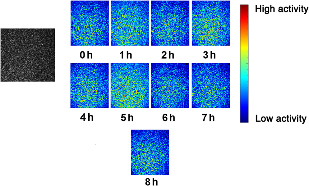
1.IntroductionDynamic laser speckle or biospeckle laser is an optical phenomenon that can be used to monitor biological and nonbiological activity in many areas.1–3 There are many ways to provide the monitoring. In some, the observed area is considered homogeneous; thus, the outcome can be summarized by a numerical index, such as in maturation of fruits4,5 or in motility of sperm6 and parasites in liquid medium, among others.7 Applications monitoring the activity in meat,8 in carrot’s respiration,9 in parasites,10 or even in cell’s culture11 are examples of the hypothesis of the homogeneity when the numerical index is adopted to quantify the activity of a material. Despite that, most phenomena, including those cited, present a level of inhomogeneity that can compromise the outcome, adopted as indirect information of a biological, chemical, or physical phenomenon. The application in cells, for instance, can be a case where the aleatory distribution of isolated cells creates clusters of different activities in the illuminated samples.12–14 The same phenomenon, linked to random movements, can be observed in microbial populations15–17 and in the transition from random to coordinated directional migration18 or even in cell division.19 Thus, despite that the study of cells and microbial population considers them homogeneous environments, reducing their complexity,20 the assumption of homogeneity cannot be applied directly to biospeckle laser monitoring of cells and microbial distribution in a medium. The main hypothesis of this work assumed that the traditional methods to analyze the dynamic laser speckle, building the time history of the speckle pattern (THSP),21,22 are compromised by the variation of homogeneity in the illuminated sample, particularly cells in a medium. Thus, the THSP, usually built by a line or a column, may not represent the sample regarding the homogeneity. This work evaluated the quality of the traditional sampling regarding the construction of the THSP and proposed a random sampling to overcome the variation of homogeneity during the dynamic laser speckle analysis. 2.Materials and Methods2.1.Preparation of Samples2.1.1.Culture of RAW 264.7 cellsFor dynamic speckle analysis, RAW cells in four wells of multiwell cell culture plates, RAW cells per well, with clear-bottom polystyrene treated with CellBIND® (Corning Life Sciences, Hazebrouck Cedex, France), were left to adhere for at least 2 h at 37°C and 5% . The room temperature was and 56% relative humidity, measured before and after the imaging.23 Four wells with the same number of cells were used, with 10 replications, resulting in a set of 40 samples. 2.1.2.Paint dryingA surface of was painted with acrylic white ink, forming a homogeneous layer. The room had 22°C to 23°C and 51% to 53% of humidity. The 10 replications were tested for each hour. 2.1.3.Coffee seed and cancer tissueThe raw data of a coffee seed24 and of a cat’s cancer tissue25 were used to evaluate the feasibility of Gaussian distribution of the selected points around an interested area. In the case of the coffee seed, the interested area was the endosperm of the seed, while the interested area in the cat’s tissue was the normal tissue surrounding the cancer tissue. 2.2.Dynamic Laser Speckle SetupFigure 1 presents the experimental setup to acquire the speckle patterns generated in time by the illumination of the samples using a linearly polarized He–Ne laser beam (632.8 nm, 30 mW). The beam size of the expanded laser light was 110 mm in diameter, presenting a monitored area of a square edge with 38 mm. The images were acquired by a compact macrolens (SIGMA) with a focal length of 50 mm, numerical aperture of (speckle size was ), connected to an Allied Vision Technologies charge-coupled diode (CCD) camera (AVT Marlin F-145B), pixel size of . 2.3.Methodology to Speckle Patterns AcquisitionIn the case of raw cells, at the beginning of each hour, during 8 h, a collection of 120 images (8 bits, , and shutter speed ) was acquired at a rate of one frame per second. While in the case of paint drying, at the beginning of each minute, during 10 min, a collection of 96 images was acquired at a rate of 15 frames per second. 2.4.Image ProcessingThe speckle patterns were analyzed by graphical and numerical indexes. The graphical index adopted was the generalized differences (GDs)26 addressed by Eq. (1). The outcomes were used to evaluate the level of homogeneity in the map of activity that can be presented in colors, with blue meaning low activity and red meaning high activity (or in gray levels, with dark gray meaning low activity and light gray meaning high activity). The numerical index adopted was the average value of the differences (AVD)26 presented as where COM is the co-occurrence matrix related to the THSP and and variables represent the line and the column of each point of the COM matrix, respectively.The construction of the THSP using the traditional selection of a line (Fig. 2) and the alternative proposal using random points in the first image (Fig. 3) was done before the adoption of Eq. (2). Fig. 2THSP methodology: (a) using the traditional selection of a row in a collection of speckle patterns in time, (b) random points in the first image (ROI) and fixed in the other images in time, and (c) of random points in the SROIs. 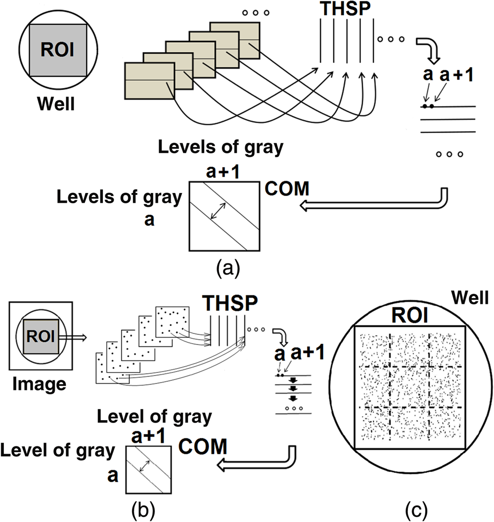 Fig. 3ROI treatment: (a) detail of the data used to construct the THSP using the random points and the selection of pixels in a line within the ROI and (b) detail of the division of subregions within the main ROI (SROI), using random points and a line within each SROI.  2.4.1.Time history of the speckle pattern by finite number pixelsBiospeckle activity in the analyzed regions of interest (ROIs) was quantified by descriptors based on temporal analysis, using the AVD method,26 after the creation of a THSP27 matrix as can be seen in Fig. 2(a). In Fig. 2(b), it is possible to see the new proposal where the THSP was created using a random number of pixels spread in the well instead of using a row, as presented in Fig. 2(a). The comparison of the traditional usage and the random points was conducted in the whole image (ROI), dividing the ROI in nine pieces [sub-ROIs (SROI)]11 as presented in Fig. 2(c). A row was also used to create a THSP in each of the nine squares, and their AVD could be compared to the proposed method based on the random assembling in the first image in time, with fixed points during the construction of THSP. In Fig. 2(d), one can see the two methods in the main ROI (whole area), and in Fig. 2(e), one can see the way the two methods were applied in the nine SROI. The size of the line in the main ROI had 244 pixels, creating a THSP of , where the value 120 represents the images collected in time, at a rate of 0.08 s. In the same way, the THSP was also constructed using the random values with , where the value 244 represents the random pixels in 120 images in time. The 244 random points selected in the first image stood still in all the images in time. The possibility of using the column instead of the line was tested, where the size of the column in the main ROI was 250 pixels. It used five lines and five columns as replications to test the variability of the traditional method. The proposed method adopted five collections of different random points to test the variability of the data. In the nine SROI, the size of the rows inside them was 80 pixels, and the THSP resulted in a size of , where the value 120 represents the number of images collected in time. The THSP was also constructed using the random values with , where the value 80 represents the random pixels in 120 images in time. The random points since selected in the first image were fixed during time. 2.4.2.Influence of the number of points in the time history of the speckle pattern constructionThe THSPs built using random points selected in the first image and fixed during time were , , , , and , with 120 meaning the number of images in time and the other dimension of the THSP related to the number of points adopted. 2.4.3.Analysis in homogenous samples—Drying paintThe test of the proposed method was conducted in samples considered with high homogeneity, in this case, of drying paint. A thin layer of ink was painted in a surface and illuminated by a He–Ne laser using a backscattering configuration as presented in Fig. 1. 2.4.4.Alternative to collect the random points—Gaussian functionsAn alternative way to create a collection of random points around a desired area is presented and named Gaussian THSP, where a circular area is defined by the radius of a Gaussian distribution. The samples elected to be analyzed were highly heterogeneous with distinct areas of activity in delimited portions of the illuminated area. A bean coffee seed and a tissue with cancer were the samples used with the selection of a point within a desired area, in this case, in a normal tissue. The Gaussian distribution of the random pixels was then around the selected point. 3.Results and Discussion3.1.Analysis of the Distribution of CellsIn Fig. 4, it is possible to see the maps of activity in wells with 200,000 cells dispersed without a defined cluster and without a homogeneous activity of the cells. The outcomes are the GDs of 128 images in time, in nine different hours. In the DGs, the activities address from blue (dark gray), representing the low activity, to red (light gray), representing the high activity of the cells. The inhomogeneity in the maps of activities presents a challenge in the numerical analysis of the biospeckle laser, when usually a line in the ROI within the wells is the source of data. For example, if you choose lines to get the pixels in the center of the wells (ROI), those lines would not always pass in the same area where the cells are expressing their activities. During 8 hours, the number of cells grew without a pattern covering the area of the wells. In Fig. 5, one can see the THSP images related to the cells samples for the traditional and proposed methods. 3.2.Numerical Analysis Using a Line and Random PointsIn Fig. 6, the AVD outcomes of the biospeckle patterns related to the wells are presented using lines of 244 pixels, columns of 250 pixels, and the same number of random points within the ROI. The adoption of lines or columns with close sizes presented significant differences in the traditional method or even when the random points were used. This reinforces the hypothesis that the set of a line of a column to get the desired information from a whole image can be done by chance and, thus, can compromise the results when inhomogeneities occur. Fig. 6Evolution of the biospeckle activity measured by the AVD index using (a) lines of 250 and 244 and (b) random points.  Therefore, the outcome of the evolution of the biospeckle activity in the cells during time, using the AVD, is addressed in the same graphic (Fig. 7) in which the difference between them regarding the variance is clear. The random points presented a smaller variance than the traditional method using the line. Fig. 7Evolution of the biospeckle activity measured by the AVD index using line with size of 244 and 244 random points in an ROI using a square inscribed in a circle, named main ROI.  Using Table 1, it is possible to see the values of the standard deviations (SDs) related to the graphics presented in Fig. 7. The SDs of the proposed method using the random points are smaller than the traditional method with the line, in accordance with the whiskers in the variance graphics (Fig. 7). The reduction of the variance, if compared to the traditional method, proves the viability of the random method of selection proposed to build the THSP and thus to analyze the assay of cells. Table 1Outcomes of AVD related to cells inside the main ROI using a line and random points to build a THSP. The outcomes are represented by the mean values of AVD and their SD with the respective percentages regarding the mean value.
3.3.Influence of the Number of Points in the Time History of the Speckle Pattern ConstructionIn Table 2, the mean values of AVD index and the random points in the main ROI to construct the THSP are increased. All the values of AVD index were done, and the mean values were obtained with the respective SDs representing their evolution with respect to the number of random points. Table 2Results of the AVD of the cells in all times representing the SD with respect to the number of points.
The stabilization of the SD can be better seen in Table 2, particularly after 20,000 random points. This means that the number of points is relevant for reducing the variation of the AVD values but with a saturation after one third of the total points are chosen. In this case, the main ROI has , and thus the number of possible points is 61,000. 3.4.Analysis in Subregion of InterestsAn alternative way to use the random points to build the THSP was the division of the main ROI in SROIs, as presented in Fig. 8, where the GD applied in the separated SROI presented different maps of activity, which proved the inhomogeneity of the sample.28 In Fig. 9, the differences observed were tested using the numerical approach (AVD), using the line and random points to construct the THSP before the AVD outcome. Fig. 9Average of the variations of the AVD of illuminated cells with the construction of the THSP, using one line and random points.  In Table 3, the values of the SD, representing the average of the nine SROI, are presented, and they are higher than the case of the main ROI (Table 1), particularly when the random points were used. The tendency of the random selection of points to reduce the variability was reinforced in the small SROI, despite the increase of the SD. Additionally, that increase was expected since the reduction of points (to 80 pixels) reduced the ability of the proposed technique to provide a dilution of the outliers. Table 3Outcomes of the mean values of the AVD related to cells inside the nine SROI using a line and random points to build a THSP. The outcomes are represented by the mean values of AVD and their SDs.
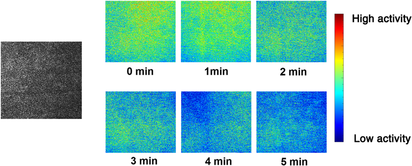
In Figs. 10 and 11, the comparison of the results of Tables 1 and 3 is presented. The comparison of the results of the AVD using the main ROI and the nine SROIs presents the higher SDs in the approach using SROIs than the main ROI when the random points were used. The comparison can be also seen when the THSP is constructed using a line in the middle of the ROI (Fig. 11). Fig. 10Variations of the AVD when the THSP was constructed using random points selected in the main ROI or in the nine SROIs.  Fig. 11Variations of the AVD when the THSP was constructed using a line of points in the main ROI or in the nine SROIs. 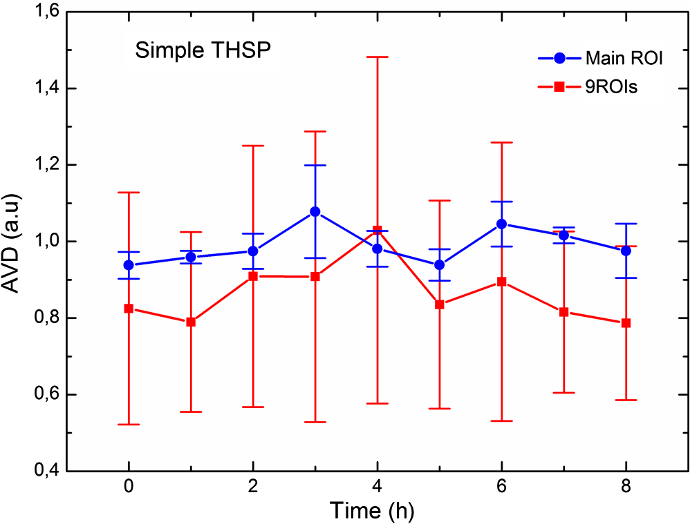 Thus, when one has samples with a level of inhomogeneity, the adoption of random points to build the THSP is the best option, and it will be better if the ROI is large enough to cover the observed sample. This method can be efficient for bacterial activity rather than the graphical methods used to monitor activities regarding the inhomogeneity of the sample.27 3.5.Analysis in a Homogenous Sample—Drying PaintThe adoption of a sample with high homogeneity than the cells was tested using the two distinct ways to build the THSP. The drying paint is usually considered homogeneous, and in Fig. 12, it is possible to see the maps of activity after the GD processing, where the magnitudes of the levels of activity in the drying paint are closer than the levels in the case of cells assay. In Fig. 13, one can see the THSP images related to the drying paint samples, related to the traditional and proposed method. The results of the adoption of the two ways to construct the THSP are presented in Fig. 14, where it is possible to see the small differences between the mean values and the variances, proving the limited efficiency of the random points to construct the THSP and to reduce the influence of nonhomogeneous areas in the monitored samples. Fig. 14Variations of the AVD when the THSP was constructed using a line of points in the main ROI and using random points in drying paint. 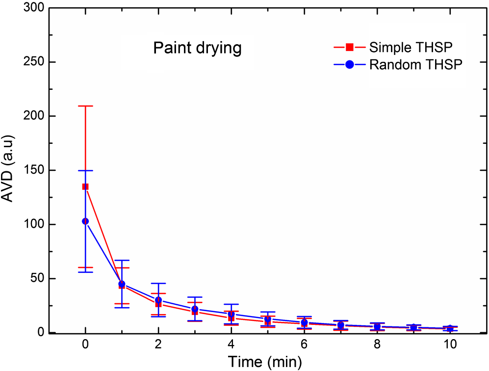 At this point, it is relevant to discuss the results involving the random points. The criteria for choosing random points instead of a simple line of points in the ROI are based on the study of nonuniform quantization of a signal.29–31 Thus, to quantize efficiently an information from a signal source (in this case, an ROI information from the pixels with intensity light values varying in time), the digitalized regions (codebook) should be based on the probability density function of the information in the ROI. In Fig. 15, the black dots represent the selection of analyzed points in an ROI and gray dots represent the interested information to be measured. In Fig. 15(a), a set of randomly selected points with a nonuniform quantization of information was used, while using a uniform probability distribution to choose the points. In Fig. 15(b), an example of uniform quantization in which the points analyzed (black points) are regularly distributed is shown. In Fig. 15(c), the classic case with a selection of points in a line is presented. Finally, in Fig. 15(d), a set of randomly selected points in a nonuniform quantization of information with the particularity that the probability density function of the spatial distribution of information is known, so the probability density function of chosen points is influenced by it is presented. Fig. 15Alternatives to analyze the biospeckle data using (a) points (codebook) selected randomly (uniform distribution) in the ROI, (b) points selected uniformly in the ROI, (c) points selected conforming a line, and (d) points selected randomly (any known distribution).  Analyzing the case in Fig. 15(c), it is easy to see that the chosen points (black) are far from the points with the interested information (gray); even if we select a different line, digitalized regions where the distance between selected and desired points will be bigger will exist, and consequently the result of processing this information will not be representative. By other side, the case presented in Fig. 15(d) has a proximity between the chosen points and the desired points; thus, these values are representatives. In this method, we need to have the information about the probability density function of the spatial distribution of the information, which is not always easy to obtain, but it is possible to make an approximation assuming that the information is distributed fulfilling a Gaussian distribution around a central point in a desired area. The alternative presented in Fig. 15(a) is the best option when the probability density function of the spatial distribution is not known (such as the case of cells monitoring) because the chosen points (black) have a good proximity to the desired points (gray) and the selection of points varies between repetitions. In this work, we presented the alternatives shown in Figs. 15(a) and 15(c). The alternative presented in Fig. 15(d) is the Gaussian distribution around a desired point, and it is useful in cases where we would like to know the activity addressed by the biospeckle laser in a well-defined area. In Sec. 3.6, one can see the case of Gaussian distribution applied in a seed and in a tissue with cancer cells. 3.6.Alternative to Collect the Random Points—Gaussian DistributionAn alternative way to select points to construct a THSP using a random distribution around a central point (pixel) is presented in Fig. 16, where the spatial probability distribution of the selected points (dots) around the chosen central pixel is defined by a Gaussian distribution, for example, if we define and as two aleatory coordinates of a random point, with probability density functions and of the variables and , respectively. In the below equation, one can have a probability density function where is the SD and is the mean value of the random variable analyzed (aka a); then, given a chosen central point , the points will be chosen following the probability density functions of Eq. (3), so the greater number of points are inside the ellipse , that is, within the ellipse with semiaxes similar to the SD.Fig. 16Coffee seed with the endosperm selected by the random points in a Gaussian distribution expressed by the dots.  In the case of Fig. 16, 200 points were chosen with a around the central pixel . Thus, with the points selected in Fig. 16, the THSP presented in Fig. 17 was formed, where it is expressed as a matrix of 200 lines and 128 columns, representing both the quantity of points and analyzed images, respectively. Finally, in Fig. 18, a Gaussian distribution in a sample where we can see that the interest region is in a specific point of the image, in this case, the normal tissue aside an area of cancer tissue is presented. Fig. 18Cancer cells aside normal tissue where the random points were collected in a Gaussian distribution expressed by the circles.  In Fig. 19, one can see the THSP image related to the tissue sample for the proposed method to illustrate the Gaussian distribution of the random points selected. 4.ConclusionsThe complex metabolism of cells was better monitored using the random points to build the THSP than the traditional case using the line of points. In the cases analyzed, the higher the inhomogeneity of the map of activity, the higher the efficiency of the proposed method using random points. Additionally, we expect that it will be the same in other nonhomogeneous samples. The proposed method can be used in different ways, such as the proposed Gaussian function around a desired area. DisclosuresThe authors have no relevant financial interests in the paper and no other potential conflicts of interest to disclose. AcknowledgmentsThe authors would like to thank the Department of Biochemistry of the Medicine and Odontology, Faculty of the University of Valencia, Spain, and the Federal University of Lavras, FAPEMIG, CAPES, CNPq, and FINEP who partially supported the work. ReferencesH. Kadono, G. Takahashi and S. Toyooka,
“Monitoring of biological activity of plant using difference-image of biospeckle,”
Proc. SPIE, 4829 988
(2003). http://dx.doi.org/10.1117/12.527504 Google Scholar
H. J. Rabal and Jr. R. A. Braga, Dynamic Laser Speckle and Applications, CRC Press, Boca Raton, Florida
(2008). Google Scholar
A. Zdunek et al.,
“The biospeckle method for the investigation of agricultural crops: a review,”
Opt. Lasers Eng., 52 276
–285
(2014). http://dx.doi.org/10.1016/j.optlaseng.2013.06.017 Google Scholar
G. F. Rabelo et al.,
“Laser speckle techniques in quality evaluation of orange fruits,”
Rev. Bras. Eng. Agríc. Ambiental, 9
(4), 570
–575
(2005). http://dx.doi.org/10.1590/S1415-43662005000400021 Google Scholar
A. Kurenda et al.,
“Effect of cytochalasin B, lantrunculin B, colchicine, cycloheximid, dimethyl sulfoxide and ion channel inhibitors on biospeckle activity in apple tissue,”
Food Biophys., 8
(4), 290
–296
(2013). http://dx.doi.org/10.1007/s11483-013-9302-7 1557-1858 Google Scholar
P. H. A. Carvalho et al.,
“Motility parameters assessment of bovine frozen semen by biospeckle laser (BSL) system,”
Biosyst. Eng., 102
(1), 31
–35
(2009). http://dx.doi.org/10.1016/j.biosystemseng.2008.09.025 Google Scholar
M. Z. Ansari et al.,
“Real time monitoring of drug action on T. cruzi parasites using a biospeckle laser method,”
Laser Phys., 26
(6), 065603
(2016). http://dx.doi.org/10.1088/1054-660X/26/6/065603 Google Scholar
I. C. Amaral et al.,
“Application of biospeckle laser technique for determining biological phenomena related to beef aging,”
J. Food Eng., 119
(1), 135
–139
(2013). http://dx.doi.org/10.1016/j.jfoodeng.2013.05.015 JFOEDH 0260-8774 Google Scholar
J. A. Alves, Jr. R. A. Braga and E. V. de B. Vilas Boas,
“Identification of respiration rate and water activity change in fresh-cut carrots using biospeckle laser and frequency approach,”
Postharvest Biol. Technol., 86 381
–386
(2013). http://dx.doi.org/10.1016/j.postharvbio.2013.07.030 PBTEED Google Scholar
J. A. Pomarico et al.,
“Speckle interferometry applied to pharmacodynamic studies: evaluation of parasite motility,”
Eur. Biophys. J., 33
(8), 694
–699
(2004). http://dx.doi.org/10.1007/s00249-004-0413-4 EBJOE8 0175-7571 Google Scholar
R. J. González-Peña et al.,
“Monitoring of the action of drugs in melanoma cells by dynamic laser speckle,”
J. Biomed. Opt., 19
(5), 057008
(2014). http://dx.doi.org/10.1117/1.JBO.19.5.057008 JBOPFO 1083-3668 Google Scholar
S. E. Murialdo et al.,
“Analysis of bacterial chemotactic response using dynamic laser speckle,”
J. Biomed. Opt., 14
(6), 064015
(2009). http://dx.doi.org/10.1117/1.3262608 JBOPFO 1083-3668 Google Scholar
S. E. Murialdo et al.,
“Discrimination of motile bacteria from filamentous fungi using dynamic speckle,”
J. Biomed. Opt., 17
(5), 056011
(2012). http://dx.doi.org/10.1117/1.JBO.17.5.056011 JBOPFO 1083-3668 Google Scholar
A. P. Vladimirov et al.,
“The use of laser dynamical speckle interferometry in the study of cellular processes,”
J. Biomed. Photonics Eng., 2
(1), 010302
(2016). http://dx.doi.org/10.18287/JBPE16.02.010302 Google Scholar
D. Lauffenburger, R. Aris and K. Keller,
“Effects of cell motility and chemotaxis on microbial population growth,”
Biophys. J., 40
(3), 209
–219
(1982). http://dx.doi.org/10.1016/S0006-3495(82)84476-7 BIOJAU 0006-3495 Google Scholar
F. W. Seymour and R. N. Doetsch,
“Chemotactic responses by motile bacteria,”
J. Gen. Microbiol., 78
(2), 287
–296
(1973). http://dx.doi.org/10.1099/00221287-78-2-287 JGMIAN 0022-1287 Google Scholar
H. C. Berg,
“Chemotaxis in bacteria,”
Annu. Rev. Biophys. Bioeng., 4
(1), 119
–136
(1975). http://dx.doi.org/10.1146/annurev.bb.04.060175.001003 ABPBBK 0084-6589 Google Scholar
C. Brangwynne et al.,
“Symmetry breaking in cultured mammalian cells,”
In Vitro Cell. Dev. Biol. Anim., 36
(9), 563
–565
(2000). http://dx.doi.org/10.1007/BF02577523 Google Scholar
R. M. Malina, C. Bouchard and O. Bar-Or,
“Growth, maturation, and physical activity,”
(2004) Google Scholar
D. Lauffenburger, R. Aris and K. H. Keller,
“Effects of random motility on growth of bacterial populations,”
Microb. Ecol., 7
(3), 207
–227
(1981). http://dx.doi.org/10.1007/BF02010304 MCBEBU 1432-184X Google Scholar
A. Oulamara, G. Tribillon and J. Duvernoy,
“Biological activity measurement on botanical specimen surfaces using a temporal decorrelation effect of laser speckle,”
J. Mod. Opt., 36
(2), 165
–179
(1989). http://dx.doi.org/10.1080/09500348914550221 JMOPEW 0950-0340 Google Scholar
R. Arizaga, M. Trivi and H. Rabal,
“Speckle time evolution characterization by the co-occurrence matrix analysis,”
Opt. Laser Technol., 31
(2), 163
–169
(1999). http://dx.doi.org/10.1016/S0030-3992(99)00033-X OLTCAS 0030-3992 Google Scholar
, “ATCC: the global bioresource center,”
(2016) https://www.lgcstandards-atcc.org/ July ). 2016). Google Scholar
P. G. Vivas et al.,
“Biospeckle activity in coffee seeds is associated non-destructively with seedling quality,”
Ann. Appl. Biol., 170
(2), 141
–149
(2017). http://dx.doi.org/10.1111/aab.2017.170.issue-2 AABIAV 0003-4746 Google Scholar
R. A. Braga et al.,
“Biospeckle numerical values over spectral image maps of activity,”
Opt. Commun., 285
(5), 553
–561
(2012). http://dx.doi.org/10.1016/j.optcom.2011.10.079 OPCOB8 0030-4018 Google Scholar
R. Arizaga et al.,
“Display of local activity using dynamical speckle patterns,”
Opt. Eng., 41
(2), 287
–294
(2002). http://dx.doi.org/10.1117/1.1428739 Google Scholar
M. Z. Ansari et al.,
“Real time and online dynamic speckle assessment of growing bacteria using the method of motion history image,”
J. Biomed. Opt., 21
(6), 066006
(2016). http://dx.doi.org/10.1117/1.JBO.21.6.066006 JBOPFO 1083-3668 Google Scholar
R. J. González-Peña et al.,
“Assessment of biological activity in RAW 264.7 cell line stimulated with lipopolysaccharide using dynamic laser speckle,”
Appl. Phys. B, 122
(11), 275
(2016). http://dx.doi.org/10.1007/s00340-016-6549-y Google Scholar
R. M. Gray and D. L. Neuhoff,
“Quantization,”
IEEE Trans. Inf. Theory, 44
(6), 2325
–2383
(1998). http://dx.doi.org/10.1109/18.720541 IETTAW 0018-9448 Google Scholar
A. Gersho,
“Quantization,”
IEEE Commun. Soc. Mag., 15
(5), 16
(1977). http://dx.doi.org/10.1109/MCOM.1977.1089500 ICSMDT 0148-9615 Google Scholar
“Vector quantization I: structure and performance,”
Vector Quantization and Signal Compression, 309
–343 Springer US, New York
(1992). Google Scholar
BiographyRoberto A. Braga, Jr. received his BA and master’s degrees in electrical engineering from Universidade Federal de Minas Gerais, Brazil, and his doctoral degree in agricultural engineering from Universidad Estatal de Campinas, Brazil. He has been a full professor at the Universidade Federal de Lavras (UFLA), Brazil, since 1996. He teaches electricity and researches in optical instrumentation. He took sabbatical leaves at BIOSS-JHI Scotland in 2005, 2008, and 2011. He has been a visiting professor at the University of Valencia, Spain, in 2014, and an external professor at Master in Medical Physics, Valencia, Spain. Rolando J. González-Peña received his master of science degree in optics from the High Technology Institute of Havana in 1998 and his PhD in technical science from the High Technology Institute of Havana in 2001. His current research is focused on digital speckle interferometry and dynamic speckle laser. Currently, he is a professor at the Physiology Department in the Faculty of Medicine and Odontology at the University of Valencia. Dimitri Campos Viana received his BA degree in control and automation engineering from Catholic University, Minas Gerais, Brazil, in 2001. He received a specialist degree in software engineering from Catholic University of Minas Gerais in 2003. He received his master’s degree in mathematical and computational modeling from CEFET-MG, Brazil, 2010. He is an assistant professor at UFLA and doctoral student in agricultural engineering UFLA, Brazil. He is experienced with control and automation engineering, working with programmable logical controllers and SCADA systems in various industries. Fernando Pujaico Rivera received his diploma degree in electronic engineering from the National University of Engineering, Perú, his MSc degree in electric engineer from the University of Campinas, and his PhD in electric engineer from the University of Campinas. Currently, he is a postdoctoral fellow with the Centro de Desenvolvimento de Instrumentação aplicada à Agropecuária, the University of Lavras, Brazil. His research interests include digital signal processing, particle image velocimetry, biospeckle laser, programming, error correcting codes, and hardware design. |
||||||||||||||||||||||||||||||||||||||||||||||||||||||||||||||||||||||||||||||||||||||||||||||||||||||||||||||||||||||||||||||||||||||||||||||||||||||||||||||||||||||||||||||||||||||||||||||||||||||||||||||||