1.

Introduction

Optical coherence tomography (OCT) is an advanced high-resolution, noninvasive imaging modality that delivers three-dimensional images from microstructures within a tissue.¹ In any OCT system, optimal transverse resolution is achievable at the focal point only. On either side of it, there is a reduction in the efficiency of the collection of backscattered light^2,3 according to the profile of the confocal gate at the core of the OCT system. The transverse resolution $\mathrm{\Delta }x$, axial resolution $\mathrm{\Delta }z$, and depth of focus (DOF) are given by the following equations:⁴

Depth selection is performed via the combined effect of the coherence gate and of the confocal gate, whose axial selection interval is determined by Eq. (3). To maximize the backscattered signal from the sample, it is necessary for the confocal and coherence gates to be aligned in depth. Using interface optics with a large NA, a high transverse resolution can be achieved. However, while improving the transversal resolution, the confocal gate interval shrinks, which leads to extension of the axial intervals where the signal is low. This makes the penetration depth shorter, unless the confocal gate is moved in synchronism with the coherence gate, a process termed as dynamic focus (DF).

To improve the transversal resolution with depth and reduce the signal decay due to the limited axial width of the confocal profile, several hardware and software procedures have been reported. As hardware procedures for Sp-OCT and SS-OCT, we distinguish multiple beam configurations and Gabor filtering. A multiple beams configuration⁶ requires multiple interferometers with different adjustments of the optical path and different interface optics focusing at different depths, i.e., a relatively complex hardware. Signals are processed in parallel, and a final image combining the best parts of cross-section images delivered by each OCT channel is stitched together in real time. With reference to Gabor filtering,⁷ the larger the NA of the interface optics, the larger the number of repetitions needed, and $R=\text{axialrange}/\mathrm{DOF}$.⁸ As documented in Ref. 9, the acquisition is repeated 10 times for a $\times 20$ magnification and 20 times for a $\times 40$ magnification. For larger NA, the number of repetitions with a focus change should be even larger. Plus, by the end of these multiple acquisitions, only the bright bands needing to be stitched together require extra time. Several configurations to adjust the focus, such as using a lens,¹⁰ a liquid lens,^7,9 or a deformable mirror,⁸ were evaluated.

Software solutions refer to deconvolution,^11–13 computational focusing microscopy techniques,^14,15 and some other image processing algorithms.^16,17 They are applicable to TD-OCT as well as to Sp-OCT and SS-OCT; however, they do not work in real time.

In this paper, a simplified procedure of DF reported earlier^18–20 is further evaluated by quantifying the signal along the depth within the images acquired. We consider that this is worth investigating due to its much simplified configuration while allowing delivery of the image in real time. DF can be applied to TD-OCT only. The DF procedure is implemented on an en-face TD-OCT scanning strategy^21–23 where both cross-section (B-scan) images as well as en-face (C-scan) images are produced based on T-scans.^24,25 These represent one-dimensional (1-D) reflectivity profiles oriented along the transversal coordinate of the object. They are orthogonal to A-scans that represent 1-D reflectivity profiles along depth, widely used by conventional OCT technology with either TD, Sp based, or SS based. Based on T-scans, the axial scanning time is reduced to that of the frame rate, which is much slower than the line rate of the conventional OCT technology based on A-scans. This relaxes considerably the technology needed for axial scanning, as recognized in Ref. 4.

2.

Principle of Operation of a Dynamic Focus Optical Coherence Tomography

With the DF scheme presented in this study, the coherence gate moves synchronously with the confocal gate peak.^18–20 The transverse resolution is then conserved throughout the scanning depth range, and an enhanced signal is returned from all depths. The synchronization of the two gates is performed by moving the microscope objective (MO) and the transversal scanning head together toward the sample. Let us consider that the two gates are superposed on top of the tissue. When the sample is moved a distance $a$ toward the OCT setup, the coherence gate moves less, only a distance $2a/n$ measured from the surface of the sample while the confocal gate moves $an$ into the sample.¹⁹ The two gates become separated in depth. The confocal and coherence gates are matched in depth when

To a good approximation, therefore, the confocal and coherence gates coincide at all depths when the refractive index of the sample to be imaged is approximately equal to 1.41. This means that any deviation from the refractive index 1.41 leads to a reduction in signal and degradation of the transverse resolution. This can be explained via a mismatch $\mathrm{\Delta }p$ of the two gates along the axial coordinate given as

Therefore, the maximum imaging range where the DF is still acceptable is obtained as

The transversal resolution at a given depth, for a gate mismatch expressed by Eq. (6), is therefore obtained as

Fig. 1

Variation of transverse resolution in depth when using the DF-OCT for imaging the tissue with an averaged refractive index of $n=1.44$. The dotted line shows the transverse resolution of the DF-OCT when a sample with the ideal value of 1.41 for its refractive index is imaged.

3.

Modifications and Improvement on the Existing Dynamic Focus Optical Coherence Tomography

Previously, we reported the design and implementation of a simplified DF-OCT at a wavelength of 830 nm.¹⁸ In this section, results are presented on a system adapted to operate at 1300 nm.

3.1.

Evaluation of Confocal Profile for Different Combinations of Collimator and Microscope Lenses

Before assembling the final DF-OCT system, an optical setup composed of a super luminescent diode (SLD) with a central wavelength of 1300 nm, a collimator, an objective microscope lens, and an optical power meter (RS1000, Newport) was assembled. This setup was used to evaluate the confocal profile for different combinations of collimator and microscope lenses with the aim to achieve the narrowest confocal gate possible (Fig. 2). Manufacturer’s specifications of the lenses are given in Table 1. A metallic mirror was used as the object, placed on a micrometer precision translation stage (M-UTM25CC1HL, Newport). The collimator and microscope lens were mounted on two XYZ translation stages. The positions of the XYZ stages were optimized manually to achieve the maximum voltage level. The mirror was moved into and away from the MO in micrometer steps using the micrometer translation stage, and the voltage on the power meter was recorded at each step. The confocal profiles measured for the combinations of collimators and MOs listed in Table 1 are shown in Fig. 3. Table 2 lists the strength of signal acquired and the width of the confocal gate in nine such combinations. To compare the efficiency in collecting the signal, the SLD was powered at $I=151\mathrm{mA}$, which delivered several mW, and the power received back was measured with the power meter. The full width half maximum (FWHM) of the confocal profiles was assessed using measurements on the oscilloscope, connected at the power meter output.

Fig. 2

Optical setup to measure the confocal profile of the single-mode fiber aperture for different combinations of collimator and MO lens as listed in Table 1. SLD, super luminescent laser diode; PC, personal computer; OF, optical fiber; and $f_1$ and $f_2$: focal lengths of the collimator and the objective microscope lens, respectively.

Table 1

Manufacturer’s specifications of the lenses used as collimator and MO in the optical setup in Fig. 2.

Lens description	Wavelength range (nm)	Focal length (mm)	Used as
Thorlabs-AR-coated aspheric lens-F280APC26	1050 to 1600	15	CL
Thorlabs-OCT Scan Lens-LSM02 $\times 10$27	$1315\pm 65$	18 ($\mathrm{WD}=7.5\mathrm{mm}$)	MO
Thorlabs-OCT Scan Lens-LSM03 $\times 5$27	$1315\pm 65$	36 ($\mathrm{WD}=25.1\mathrm{mm}$)	MO
Thorlabs-IR Achromatic doublet- AC 127-019-C-ML28	1050 to 1620	19	MO
Thorlabs-IR Achromatic doublet- AC 127-25-C-ML28	1050 to 1620	25	MO
Thorlabs-IR Achromatic doublet- AC 127-30-C-ML28	1050 to 1620	30	MO
Thorlabs-IR Achromatic doublet- AC 127-35-C-ML28	1050 to 1620	35	MO
Thorlabs-IR Achromatic doublet- AC 127-40-C-ML28	1050 to 1620	40	MO

Note: WD stands for working distance.

Fig. 3

Confocal profiles obtained from combinations of collimators and MOs listed in Table 1, using the translation stage in Fig. 2.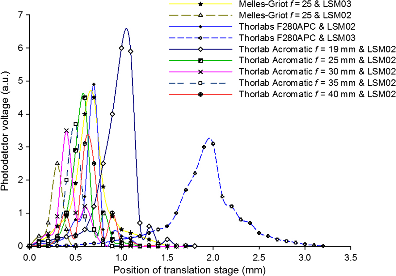

Table 2

Efficiency of signal collected and confocal width profile for the combination of elements listed in Table 1.

Configuration (using the following as, respectively, CL and MO)	Output power (μW) (at I=151  mA)	Confocal gate (μm)
Melles-Griot lens $f=25$ and LSM03	42	250
Melles-Griot lens $f=25$ and LSM02	21	110
Thorlabs F280APC and LSM02	48	100
Thorlabs F280APC and LSM03	58	450
Thorlabs achromatic lens $f=19\mathrm{mm}$ and LSM02	23	270
Thorlabs achromatic lens $f=25\mathrm{mm}$ and LSM02	16	200
Thorlabs achromatic lens $f=30\mathrm{mm}$ and LSM02	11	150
Thorlabs achromatic lens $f=35\mathrm{mm}$ and LSM02	12	115
Thorlabs achromatic lens $f=40\mathrm{mm}$ and LSM02	9	120

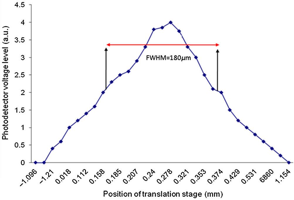
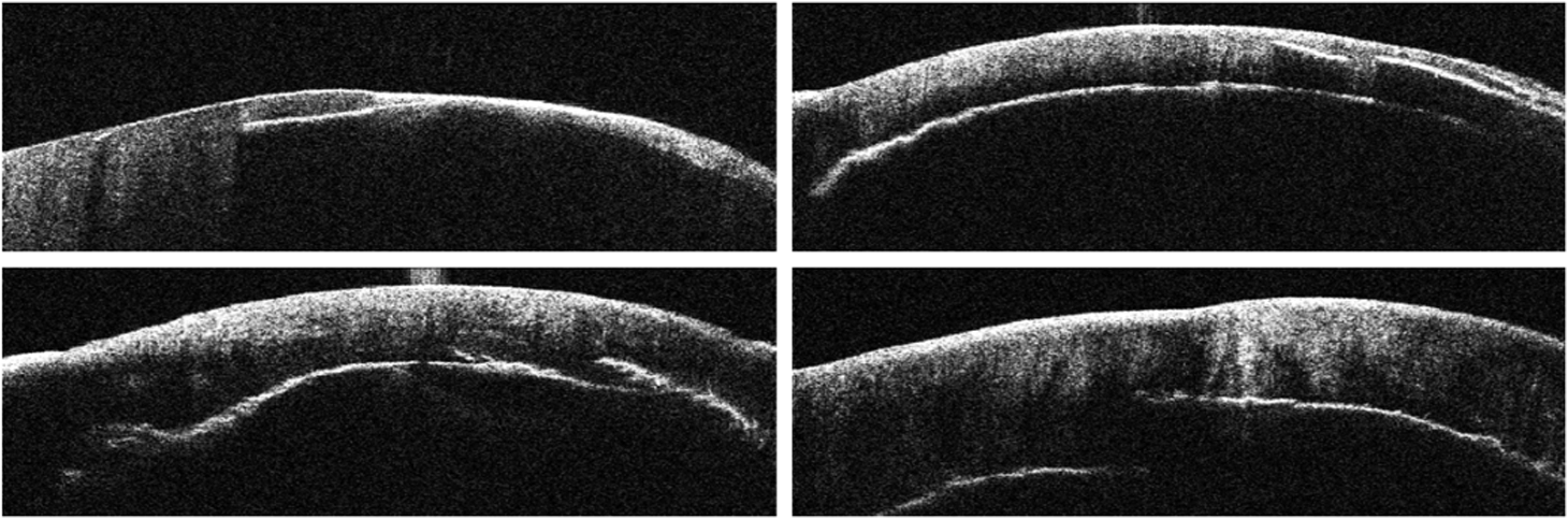
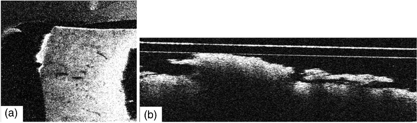
The combination of Thorlabs F280APC and LSM02 was chosen as the best out of the nine listed configurations. This combination produced the narrowest confocal gate with a loss only slightly larger ($48\mu \mathrm{W}$ measured) than the best measured ($58\mu \mathrm{W}$). We know that the LSM lenses are specially designed objective lenses by Thorlabs to perform as telecentric lenses that maintain uniform spot sizes within the scanned area. In particular, LSM02 is equipped with an antireflection coating and has been designed as a telecentric lens that maintains a uniform spot size over a 15-deg scan range. The mean spot size is $13\mu \mathrm{m}$ when the whole diameter of the lens is illuminated. It looks like the combination of Thorlabs F280APC and LSM02 delivers beams with minimum aberrations.

3.2.

Experimental Setup of the Modified Dynamic Focus Optical Coherence Tomography

A DF-OCT setup usually requires two micrometer precision translation stages, one in the reference arm and one in the sample arm. Using two translation stages in the construction of the DF-OCT systems enables synchronous scanning of the coherence and confocal gates. However, using two stages leads to synchronization complexity. Previously, Schmitt et al.²⁹ proposed a single stage. In their configuration, both the reference and object beams are run along the stage, and its optics are complex. Following the work,^18,19 in the DF arrangement that we present here, there is only one translation stage used in the sample arm. This makes the implementation of the DF-OCT simpler and the cost of the implementation much less. Such a procedure eliminates the need for synchronization of two mechanical means to move the coherence gate and confocal gate in synchronism.^23,30

The optical source used in the configuration of our DF-OCT is a Superlum SL-65-5, which is made of two SLDs emitting at 1299 and 1326 nm, combined via a coupler inside the source. The typical optical power of the SLD is 20 mW. The measurement of the optical source spectrum is performed with a commercial optical spectrum analyzer (HP 70950B). The recorded individual output spectra of the two SLDs are presented in Fig. 4(a), and the fiber-coupled output spectrum of the SLD source and its Gaussian fit are shown in Fig. 4(b). The bandwidth of the Superlum source was measured at 54 nm; hence, the theoretical axial resolution of the system in air is obtained using Eq. (1) as $\sim 14\mu \mathrm{m}$.

Fig. 4

Power spectral density of the Superlum source: (a) individual output spectra of the two SLDs and (b) fiber-coupled spectrum of the SLD output and its Gaussian fit.

The optical components used in the construction of DF-OCT are shown in Fig. 5.

Fig. 5

DF-OCT setup. BOS, broadband optical source; MO, microscope objective; CL, collimator lens; (MO and CL were chosen based on the optimization using the setup in Fig. 2); M, mirror; XY, transversal Galvo scanning head; C1, C2: $2\times 2$ couplers; OF, optical fiber; PC, personal computer; BD, balance detection receiver; CL1,2, collimator lenses; MPC, Galvo-mirror positioning controller; PCR, polarization controller; MTS, motorized micrometer translation stage that accomplishes both depth scanning and DF; and SC, stage controller. The glass rod used in the reference arm is to compensate for the dispersion.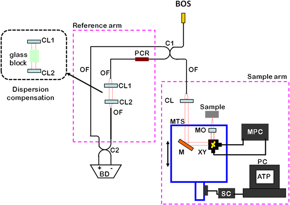

As shown in Fig. 5, light is launched from the SLD. The light is split by a $2\times 2$ coupler, C1, and enters the reference and the sample arms by a ratio of 80/20. In the sample arm, light is collimated by a collimator lens (CL) and hits the mirror. The mirror (metallic mirror), XY scanner, and MO are mounted on the motorized micrometer translation stage (M-UTM25CC1HL, Newport). Care was taken in selecting a stage with low yaw and pitch to not disturb the OCT signal. No lateral displacement of pixels in the images was noticed when shifting this stage. The mirror directs light to the XY scanner pair, which is controlled by a mirror positioning controller (MPC) device (Cambridge Technology, 6215). The line scanner in the galvo-scanning pair is driven by a triangular signal at 500 Hz while the vertical (frame) scanner is driven by a saw-tooth at 2 Hz. In this way, en-face images of 500 lines are obtained. A similar number of lines is obtained in the cross-section images as the translation stage is moved slowly in 0.5 s for the duration of image acquisition. The light is then focused on the sample using the MO microscope, LSM02. The signal returned from the sample arm is transferred via the MO and CL back to the object arm fiber and interferes with the reference signal in the reference arm. In the reference arm, the ends of the fibers can be moved by two XYZ optical translation stages. The reference arm length is adjusted initially by the gap between the stages (between CL1 and CL2). CL1 and CL2 are used to collimate the light into the fibers. The object fiber and the collimator, CL, F280APC, are moved together. To compensate for dispersion due to the optical path difference in the sample and reference arms,²⁹ two slabs from Thorlabs, made up of the same glass used in the manufacturing of the MO lens, are placed in the reference arm between CL1 and CL2 (as shown in the inset). A polarization controller (PCR) is used in the reference arm for polarization adjustment. The interference signal is produced at the 50/50 coupler C2 and is split into two ports feeding a balance detection (BD) unit to reduce the excess photon noise. The BD unit (designed at the University of Kent) consists of two InGaAs pin photodiodes with differential electronics, where the gain on one of the photodiodes is changed to balance the voltage collected from them. The signal generated by the balance detector is then recorded by a computer interface to generate the OCT image. The XY galvo-scanning mirrors, in the system in Fig. 5, slightly clip the beam; therefore, we remeasured the confocal profile. To this goal, the XY scanners were driven with zero volts, and the graph in Fig. 6 was obtained. This shows the photodetector voltage level versus the position of a mirror used as a sample. The FWHM of the confocal gate was obtained as $180\mu \mathrm{m}$. The optical power loss when traveling through the optical devices in the object arm, including the XY scanners, the mirror, collimator, and the MO lens, was measured as 16.8% each way. The loss might be due to the aberrations introduced by the mirror M and the limited aperture of the galvo-scanners.

Fig. 6

Confocal profile of the interface optics in the DF-OCT in Fig. 5.

The optical power in the reference arm was optimized by adjusting the lateral position of the XYZ translation stage. The sensitivity of the DF-OCT was then measured as 85 dB.

3.3.

Images Produced by the Dynamic Focus-Optical Coherence Tomography

The DF-OCT system was used for imaging different samples, such as fingertip skin, epoxy resin phantoms, teeth, and larynx tissue. In Fig. 7, a B-scan image of a fingertip of a 28-year-old Asian male is shown. The B-scan and C-scan images of a phantom composed of gold microspheres ($\text{average size}=4\mu \mathrm{m}$) embedded in the mixture of the epoxy resin and hardener³¹ are shown in Figs. 8(a) and 8(b), respectively. Evaluation of the transversal resolution of the system is performed in Fig. 8(c). In Figs. 9 and 10, B-scan and C-scan images of a human tooth are presented. B-scan and C-scan images of larynx tissue in vitro are shown in Fig. 10. For each of the images in Figs. 7, 10, and 11, ethics approvals were obtained, in conjunction with collaborators.

Fig. 7

B-scan image of a fingertip of a 28-year-old Asian male (type II). Image size is $4.5\mathrm{mm}\times 1.5\mathrm{mm}$. In this image, skin layers are distinguishable, and sweat ducts are identified by white arrows.

Fig. 8

Images of a phantom composed of gold particles ($\text{average size}=4\mu \mathrm{m}$), embedded in epoxy-resin. (a) B-scan image, 4.5 mm (lateral) $\times 1\mathrm{mm}$ (measured in air), (b) C-scan image, $3.5\mathrm{mm}\times 3.5\mathrm{mm}$ lateral size, and (c) transversal resolution of the DF-OCT system evaluated on the scattering center in the red dotted box in (a).

Fig. 9

B-scan images of an extracted tooth at different transverse positions. Size of the images is $4.5\mathrm{mm}\times 1\mathrm{mm}$.

Fig. 10

C-scan images of an extracted tooth at different depths. Size of the images is $4.5\mathrm{mm}\times 4.5\mathrm{mm}$.

Fig. 11

Images of larynx tissue. (a) C-scan image of larynx tissue and (b) B-scan image of the larynx tissue.

4.

Validation of Dynamic Focus Concept

A solid transparent homogeneous phantom composed of ${\mathrm{TiO}}_2$ particles embedded in epoxy-resin with a concentration of 12% was constructed. The epoxy-resin was obtained by combining Araldite DBF and AraDVR hardener (XD716). The details of the construction of the phantom are given in Refs. 31 and 32. B-scan images were collected from the phantom at different positions of the coherence gate while the focus was set on the surface of the phantom. The images are shown in Figs. 12(a), 12(b), 12(c), and 12(d). The results of this experiment showed that as the coherence gate approaches the peak of the confocal gate, the signal to noise ratio (SNR) of the image increases, as shown in Figs. 12(a), 12(b), and 12(c). The image becomes brighter throughout its depth range when the coherence gate and the peak of the confocal gate are completely matched [Fig. 12(d)].

Fig. 12

Four B-scan OCT images of a homogeneous solid phantom composed of ${\mathrm{TiO}}_2$ particles embedded in epoxy-resin. The coherence gate moved toward the surface of the sample. The surface of the sample was in focus. The confocal and coherence gates are separated by: $d=0.5\mathrm{mm}$ in (a), 0.25 mm in (b), 0.1 mm in (c), and 0 in (d) (the two gates matched). Size of the images is $2\mathrm{mm}\times 1\mathrm{mm}$.

The images in Fig. 12 are linear gray level images. A rectangular area of $25\times 195\text{pixels}$ in the images, as shown in Fig. 12(c), along the axial direction is considered. A two-dimensional smoothing filter is applied to this area to soften the selected region. The horizontal pixels are then averaged, so an averaged smoothed A-line is obtained. The A-line associated within such rectangles placed above the images in Figs. 12(a), 12(b), 12(c), and 12(d) is shown in Fig. 13.

Fig. 13

A-lines associated with the images in Fig. 12. Trendline is computed for the part of each A-line that is inside the phantom for four mismatch cases: (a) 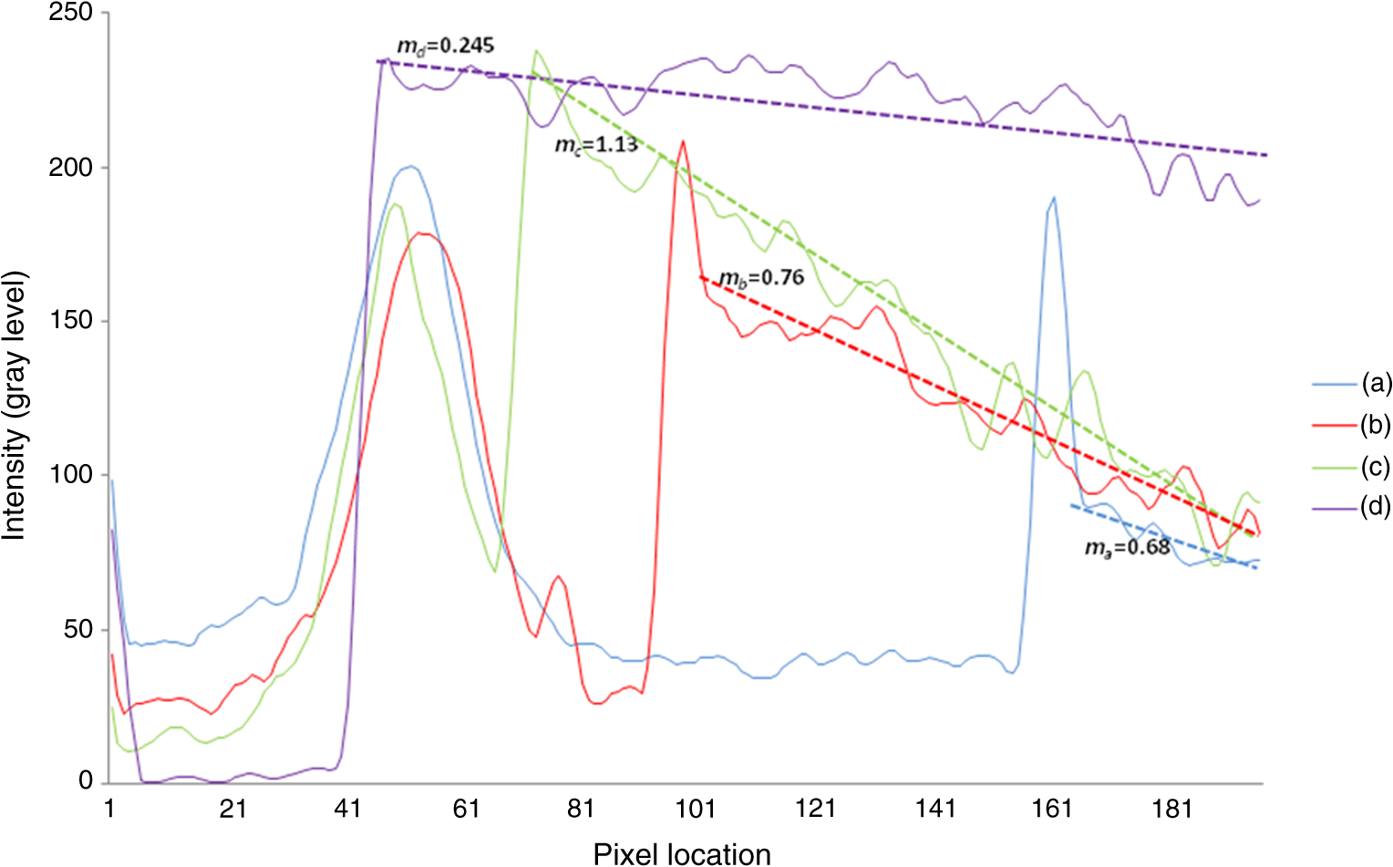$d=0.5\mathrm{mm}$, (b) $d=0.25\mathrm{mm}$, (c) $d=0.1\mathrm{mm}$, and (d) $d=0$.

The “trendline,” a built-in function in Excel, was used to depict decay/trend in the part of the A-line that is within the sample. The absolute gradient for the trendlines is calculated. The gradient of the decay represents the attenuation due to the combined effect of the confocal gate and of the absorption/scattering within the tissue. The results of this experiment showed that as the coherence gate approaches the peak of the confocal gate, the decay increases from 0.68 to 1.13. This is due to the fact that the coherent gate is moved from a relatively constant but small efficiency (away from focus) region of the confocal gate to a region of large variation when close to its maximum. However, when the confocal and coherence gates are matched, the slope of the decay dramatically reduces to 0.245. The decay left is exclusively due to the absorption/scattering of the sample.

In another experiment, the performance of the DF-OCT is compared to that of a SS-OCT.³³ The SS-OCT system consists of the same optical setup used for the DF-OCT; however, the SLD is substituted by an SS (Axsun 1310 Swept source, manufactured by Axsun Technologies) and the signal acquisition hardware changed accordingly. A fast photodetector is used, and the motorized moving translation stage is held the same. The SS has a tuning bandwidth (10 dB) of 106.0 nm (1256.6 to 1362.8 nm). This determines an axial resolution of $5\mu \mathrm{m}$ using Eq. (1).

A phantom composed of super white polyester microspheres embedded in the same epoxy-resin used in the previous experiments was constructed and imaged with both SS-OCT and DF-OCT. A B-scan image of the phantom obtained by the DF-OCT is shown in Fig. 14.

Fig. 14

(a) B-scan image of the phantom composed of super white polyester microspheres embedded in epoxy-resin and hardener, (b) relative transversal resolution range along the rectangles 1, 2, and 3. Image size is $2.5\mathrm{mm}\times 1\mathrm{mm}$. The rectangular areas 1, 2, and 3 are the representative areas from which the transversal resolutions have been calculated.

The same phantom was imaged for different positions of the confocal gate by an SS-OCT system operating at 10 kHz, with a sensitivity exceeding 92 dB. The B-scan images are given in Fig. 15 for four different positions of the confocal gate. In Fig. 15(a), the focus is placed just above the sample. The confocal gate was then moved in steps of $200\mu \mathrm{m}$ inside the sample. In Figs. 15(b), 15(c), 15(d), and 15(e), the focus was moved to 200, 400, 600, and $800\mu \mathrm{m}$ away from the surface of the sample, respectively.

Fig. 15

SS-OCT B-scan images of a phantom composed of super white polyester microspheres embedded in epoxy-resin. Image size is 1.5 mm (lateral) $\times 2\mathrm{mm}$ (vertical, measured in air). OPD is zero. (a) Focus is on the surface of the sample, (b) focus is $200\mu \mathrm{m}$ inside the sample, (c) focus is $400\mu \mathrm{m}$ inside the sample, (d) focus is $600\mu \mathrm{m}$ inside the sample, (e) focus is $800\mu \mathrm{m}$ inside the sample, and (f) relative transversal resolution range along the rectangular areas 1 and 2 specified on (e). The rectangular areas 1 and 2 are the representative areas from which the transversal resolutions (in focus and out of focus) are calculated.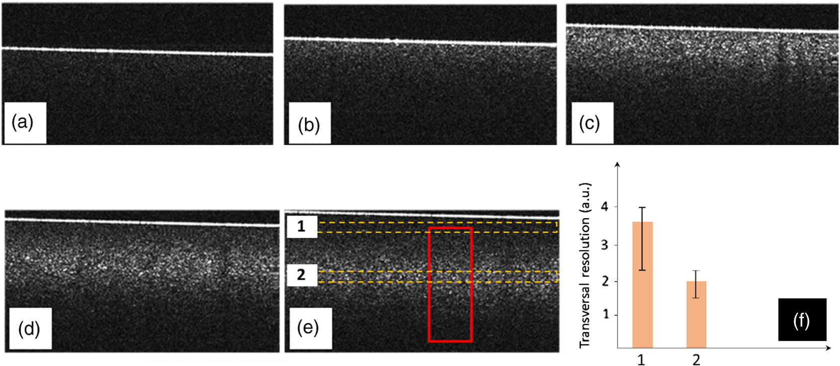

Visual comparison between the images collected from the DF-OCT and SS-OCT shows that the intensity decay in SS-OCT decreases the SNR of the regions other than those close to the peak of the confocal gate. In contrast, the intensity decay in the DF-OCT images in Figs. 12(d) and 14(a) is not noticeable at all. It was mentioned earlier that the confocal gate of the DF-OCT was measured as $180\mu \mathrm{m}$. From the image in Fig. 15(e), the confocal gate of the system was calculated again as $200\mu \mathrm{m}$ (Fig. 16).

Fig. 16

Averaged smoothed A-line intensity profile of the image given in Fig. 15(e) (red rectangle). The confocal gate computed from the profile is $200\mu \mathrm{m}$.

In terms of transversal resolution, this is almost constant in Fig. 14(a), as shown in Fig. 14(b) along the depth, while varying with depth as expected in Fig. 15(f). We should also expect an increase in the FWHM for the transversal resolution results attributed to the wavefront distortion through the intermediate layers.

5.

Conclusions

We presented the implementation and the related theory of the DF-OCT. The system was then evaluated on several samples. The DF-OCT configuration has the following specifications: lateral resolution between 8 and $9\mu \mathrm{m}$, axial resolution of $9.6\mu \mathrm{m}$ (in tissue with $n=1.44$) based on the spectral width of the SLDs, $\mathrm{\Delta }\lambda =54\mathrm{nm}$, optimized confocal gate of $180\mu \mathrm{m}$ (measured in air), capability to image tissues with a C-scan size up to $5\mathrm{mm}\times 5\mathrm{mm}$ and a B-scan size up to $5\mathrm{mm}\times \mathrm{mm}$ (measured in air), with better than 85-dB sensitivity. The system was used to successfully image different samples, such as fingertip skin, several epoxy-resin phantoms, a human tooth, and larynx tissue.