|
|
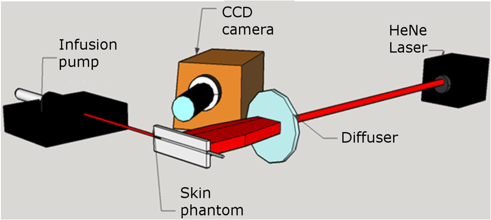
1.IntroductionThe visualization of blood vessels is of fundamental importance for a wide variety of biological and biomedical applications, such as obstruction, stiffness, and response to an external stimulus. Laser speckle imaging (LSI) is a technique based on the spatial–temporal integration of the light scattered from a biological sample when illuminated with coherent light and imaged by an optical detector (i.e., CCD camera).1,2 Particle motion (i.e., blood cells) in the illuminated area causes a decrease in contrast, seen as a blurring effect in the image, which is related to the speed of the particles in the illuminated sample. Hence, LSI is used to measure the relative blood flow speed.3,4 For deep vessels, LSI shows some limitations5 because of the strong scattering produced by static structures, such as the skull or the epidermis. Several approaches have been proposed to overcome these limitations. Pulsed photothermal radiometry (PPTR) photoinduces heating in blood vessels with a laser pulse to improve the visualization.6 Photothermal-LSI is a recently developed technique that combines the photoinduced heating of PPTR and the contrast of integrated intensity of LSI to improve the visualization of the deep blood vessels.7 Magnetomotive laser speckle imaging uses paramagnetic nanoparticles introduced in the vasculature. Under the influence of an external magnetic field, the mobility of those particles increases, allowing their visualization through the contrast of integrated speckle.8 Physicochemical tissue optical clearing (PCTOC) uses a topical substance that matches the refractive index of the skin.9 Although these techniques may increase the visualization of the deep blood vessels up to a few hundred micrometers, all of them require an external agent or stimulus. In a recent work, Postnov et al.10 proposed a computational algorithm based on a second-order gradient that allows vessel location and measurement of its diameter from the contrast speckle images. However, the algorithm was applied to a relatively superficial vessel. In this work, we present a noninvasive technique to improve the visualization and location of deep vessels in skin phantoms through digital image processing of raw speckle images (RSI). The approach consists of: (a) processing the RSI as texture images to obtain its homogeneity representation through the co-occurrence matrix (CM) and (b) automatically locating the vessel through a kurtosis analysis. Kurtosis has been used in other approaches to study the speckle patterns produced by the surface’s roughness,11,12 but here, kurtosis is used to estimate the vessel location and its diameter in an automatic way. Results of the homogeneity representation are compared with a standard LSI image. In addition, the accuracy of this methodology is demonstrated by estimating the vessel diameter at different depths. The proposed kurtosis analysis was compared with the full width at half maximum, demonstrating that the former can provide more accurate results. The sections of this work are divided as follows. In Sec. 2, materials and concepts used in this work are described. Section 3 describes the proposed methodology. In Sec. 4, the obtained results for different sets of RSI are presented. Finally, the conclusions and the future work are presented in Sec. 5. 2.Materials and Methods2.1.Texture and Co-occurrence MatrixIn computer vision, a texture is characterized by gray-level variations in an image that form small similar and repetitive regions.13 Thus, in order to describe a texture, it is necessary to analyze the distribution of its gray levels. While a histogram provides information about the distributions of gray levels, it does not take into account the relationship between a central pixel and its neighbors.14 This information is important to provide a rich description of the texture. The gray level CM is one of the standard methods to analyze texture in digital image processing13 and can be used for describing the information of RSI, as we report in an initial approach.15 Through second-order statistics, this approach studies the way in which the gray levels are distributed in an image or region and their spatial relationships.16,17 A CM indicates the frequency at which a pair of pixels with gray values and , located spatially at a distance of pixels in the direction , occurs in an image . A distance value must be chosen carefully because a large distance may result in texture overlapping; oftentimes, is used. The analysis direction takes values of ; the analysis in all the directions is obtained by the addition of the four matrices. Let be a pixel in the image of rows and columns, where takes gray values in the range , being the range of possible values (256 for an 8-bit image). For instance, if is an image with five possible gray values from 0 to 4 (), as shown in Fig. 1(a), and the parameters and are considered for its CM, then the procedure is as follows. A matrix is generated and set to zeros; CM is always square and its dimensions depend on . To assign values to the CM, each pair of pixels in is analyzed considering the parameters and . Figure 1(b) shows that for the central pixel , the parameters indicate that is the neighbor pixel to analyze. Often, the neighborhood analysis is made symmetrically; hence, the cooccurrence is also extended to . Suppose we want to know the cooccurrences of a gray level (reference level) with a gray level (comparison level), denoted as . For , the cooccurrences with happen when the coordinates of are , therefore . For , the cooccurrences with happen in coordinates by considering a neighborhood in . Also, in this case, the cooccurrences happen in a symmetrical way, when has coordinates by considering a neighborhood in ; therefore, . The final CM is obtained by analyzing the cooccurrences between all the possible values of and , as shown in Fig. 1(c) for this example. Fig. 1(a) Example of a small image with , (b) the neighborhood for cooccurrence analysis, and (c) its resulting CM. 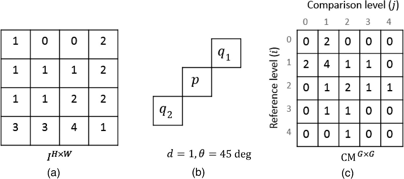 From the CM calculus, two important things should be noted: (a) a new representation of the gray levels in is provided by the CM, which is considered a symmetric two-dimensional histogram, but it does not characterize a texture by itself;13,18 (b) although the amount of information in has been reduced in the CM, a large amount of data remain for texture characterization, i.e., characteristics. 2.2.Feature ExtractionIn order to use the information provided by the CM, some features must be calculated. Haralick et al.17 proposed 14 textural features that can be calculated from the CM to identify difference among textures. One of the most used features is the inverse difference moment, a measure of the local homogeneity, calculated as where is the probability density function obtained by dividing the CM matrix by the total pixels of image (); and are the reference and comparison levels of the CM matrix described in Sec. 2.1.19,20 This feature provides information regarding the differences between gray levels in the image, taking values in the range [0, 1], where 1 indicates a limited range of gray levels (high homogeneity) and 0 indicates a wide diversity of gray levels (high roughness). For instance, texture T1 in Fig. 2(a) contains coarse structures (bricks) identified by having close gray values and smooth transitions among them. Thus, high occurrences are expected near the CM diagonal of this image with . In the opposite case, when an image contains fine granulated structures (T2), the scattered occurrences are expected throughout the CM, as in the case of Fig. 2(b), and consequently, a lower homogeneity . Thus, it is possible to find differences among textures by calculating features, such as homogeneity based on the CM values.2.3.Skin PhantomsThese skin phantoms consist of two parts: dermis and epidermis with specific characteristics, as suggested by Saager et al.21 For the dermis phantom [Fig. 3(a)], we used a transparent resin with the necessary amount of titanium dioxide ( ) to simulate the scattering coefficient of the skin (). The epidermis phantom [Fig. 3(b)] was made of silicone (polydimethylsiloxane) mixed with powder () to simulate the corresponding scattering properties () and dried coffee () to simulate the absorption coefficient ().21 Different thicknesses of phantom epidermis layers, namely 200, 400, 500, 600, 700, and , were placed on top of the phantom dermis to simulate different depths of the vessels [Fig. 3(c)]. 2.3.1.In vitro vesselsFor this work, two types of in vitro vessels were used: straight and bifurcated. For the straight vessel, a glass capillary with an inner diameter of was used, whereas for the bifurcated vessel, a slide with -inner diameter microchannels (thinXXS Microtechnology AG, Germany) was used. Both in vitro vessels were placed above silicon layers containing powder to mimic the scattering properties of the soft biological tissues. The phantoms described in Sec. 2.3 were placed on top of the slide to simulate the depth of the vessels [Fig. 3(c)]. 2.4.Experimental SetupThe LSI setup (Fig. 4) consists of laser He–Ne (632.8 nm) that impinges on a static engineered diffuser (Model ED1-C20, Thorlabs Inc.), which in turn illuminates homogeneously a circle with a 1-cm diameter on the phantom’s surface. If the phantom is not homogeneously illuminated, the intensity distribution can influence the corresponding spatial contrast. A lens coupled to a CCD camera (Model Retiga 2000R, QImaging, Canada) images the surface of the phantom on the CCD. The magnification of the optical system is and the corresponding speckle size is . Alinear polarizer is placed in front of the lens with its transmission axis crossed with the He–Ne polarization to minimize the specular reflection. The CCD camera is connected to a computer to save the captured speckle images. The camera exposure time is set to because this value is quite common for in vivo LSI applications.22 This exposure time is approximately three-orders of magnitude larger than the correlation time reported23 for a similar LSI experiment at a flow speed of . An infusion pump (Model NE-500, New Era Pump System Inc.) was used to inject the intralipid at 3% in water as blood substitute, whose scattering coefficient is at 630 nm.24 The pump allows control of the speed of the intralipid through the glass capillary. In this work, we use two different flow speeds: 10 and . A similar range of speeds has been used in similar experiments.25 3.Proposed Methodology for Automatic Vessel LocationThis proposal addresses the analysis of an alternative representation to the traditional contrast representation in a laser speckle. In order to compare both representations, an introduction to the known contrast representation is first given. 3.1.Contrast RepresentationBriers and Fercher26 demonstrated that it is possible to estimate the relative blood flow speed from the blurring (contrast) of a spatial and temporal integrated speckle pattern. The contrast measure () is defined as the ratio between the standard deviation () and the mean intensity gray value () over a sliding window in the image [Eq. (2)]. Low values of indicate a reduced range of gray levels (smoothness), whereas high values of indicate a high dispersion among the gray levels (variability). The contrast highlights the difference between static (skin) and dynamic (blood vessel) regions of an RSI (Fig. 5), improving their visualization (contrast representation). As shown in the two views of the LSI [Figs. 5(b) and 5(c)], the contrast changes abruptly in any given region, which may hinder vessel boundaries location, and this task becomes harder as the depth increases. In a blood vessel location task, this is a drawback because it implies that vessel limits become harder to define as the depth increases. Therefore, in this work, we propose the use of a homogeneity descriptor based on a CM computing that not only takes into account the spatial relations among gray values but also provides a representation that is less sensitive to the variability of the speckle pattern. This is an important characteristic as it provides a better definition of the vessel location, as described next. Fig. 5(a) An RSI of a superficial vessel (i.e., ) and (b, c) its contrast image computed with an analysis window of . The homogeneity computed images using analysis windows of (d, e) and (f, g) , respectively. Left and right columns show the transversal and frontal views of the images, respectively. 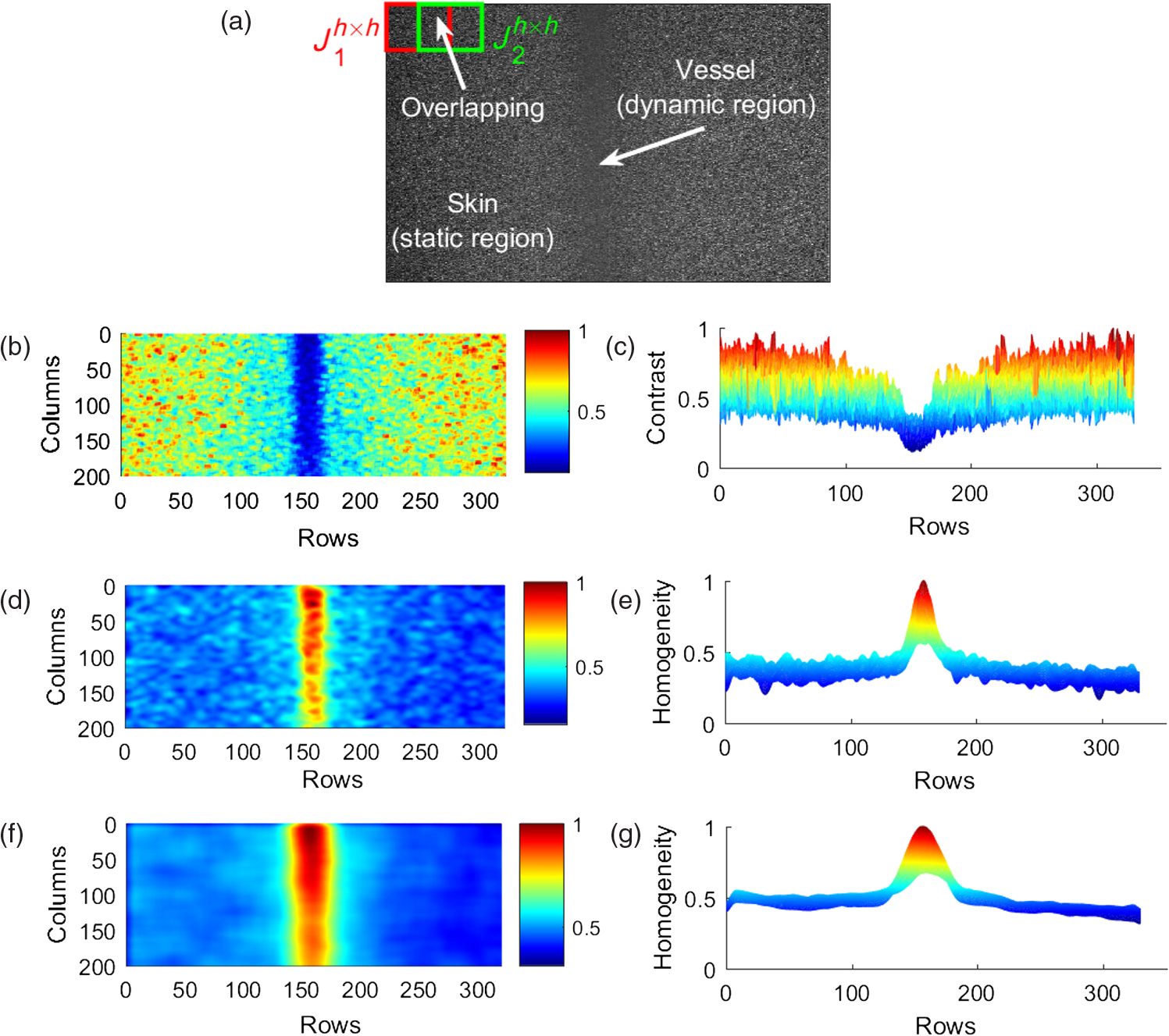 3.2.Homogeneity RepresentationIt must be taken into account that the vessel region usually occupies a small area in the image; therefore, the homogeneity value must be computed for the small regions. Hence, the image is divided into subimages or subregions through an analysis window [Fig. 5(a)], and a CM is calculated for this area, just as the contrast image is calculated. With the aim of increasing the precision in the location of the vessel, a certain level of information redundancy is necessary. There must be an overlap between each pair of subregions, i.e., must have a displacement with regard to with where is the size of the analysis window. In this way, we generate a new representation of the RSI through the homogeneity image, shown in Figs. 5(d) and 5(e), in which it is possible to improve the discrimination between dynamic and static regions. As shown, high and low values of homogeneity will be associated to dynamic and static regions, respectively. Homogeneity representation enables smoother transitions among consecutive regions and defines the vessel better. Often, the analysis window has a small size, such as or , but if a large area is analyzed, it is possible to find statistics that better describe the characteristics of that area. This is particularly interesting because the speckle pattern is generated randomly. If the analysis is made using a small window, a higher dispersion is found [as shown in Figs. 5(b)–5(c) and Figs. 5(d)–5(e)]; but if a larger window is used, that dispersion is attenuated because the occurrence of gray levels becomes higher, i.e., some of them are no longer seen as isolated occurrences and the relationship among pixels is higher, although they still reflect local values. As the use of a larger window improves the homogeneity representation by avoiding strong variations, the use of a larger window with and will be explored. As shown in Figs. 5(f) and 5(g), the use of a larger window improves the homogeneity representation by avoiding strong variations. The transversal view of (, hereinafter named as homogeneity profile) shows with more detail that low homogeneity values are related to static region, whereas high homogeneity values are related to dynamic regions, i.e., regions of high contrast. We can also observe that the homogeneity rapidly increases in the regions closest to the vessel until it reaches its maximum level at the center of the vessel. In this new representation, it is clearer to distinguish the static and the dynamic regions, thereby improving the vessel location. Although this homogeneity profile corresponds to an RSI at in depth (which we call the reference case), this analysis can be extended to deeper vessels. 3.3.Homogeneity Profile CharacterizationIn LSI, it is known that the vessel region is associated with a blurring effect due to the blood flow (dynamic region);1 however, as the depth increases, this effect is reduced, making it difficult to identify the vessel region. Although a certain level of blurring remains in the image, the dynamic region becomes very similar to the static region. Therefore, we need to find other ways to identify the vessel region from an image that appears to be completely noisy. The homogeneity representation will be used for this purpose. For the proposed methodology, an initial set of RSI (S1) was tested. The set contains a package of images obtained using the experimental setup described in Secs. 2.3 and 2.4. Table 1 describes the characteristics of this package, consisting of 30 RSI images at in depth. This is done in order to study whether there is a characteristic pattern in the homogeneity behavior. The starting point (reference case) is . All the homogeneity profiles were found to present a distribution with a tall narrow peak and long tails due to the extreme deviation from the central tendency of the values, this feature suggest the use of kurtosis. This deviation was caused by the rapid increase of homogeneity values in the dynamic region [similar to Figs. 5(e)–5(g)]. Table 1Characteristics of the reference set (S1) of RSI.
The kurtosis is a measure that describes the shape of a distribution based on the ratio between the central tendency and the deviation of the data.27 When values are greatly deviated from the central tendency, the kurtosis takes values , and the distribution is called leptokurtic. Given that a superficial vessel at has a characteristic leptokurtic homogeneity distribution, kurtosis can be used as a parameter of reference for vessel location. In order to prove this statement, the kurtosis value () was calculated for the 30 profiles, according to where is the fourth moment about the mean, i.e., the sum of the difference between the mean and each value raised to the fourth power in a given set of values; is the standard deviation. The obtained mean kurtosis () of the reference case is confirming its leptokurtic distribution (Table 1). In order to determine the quality of the set S1, the peak signal-to-noise ratio (PSNR) for all RSI images of S1 was estimated using where is the mean value of the image .28 The images of S1 were found to have a high PSNR; therefore, we use its mean kurtosis value as a reference for the proposed analysis.Once the reference homogeneity profile has been established, it is necessary to locate the vessel and later to estimate its diameter, as shown in Sec. 4.1. A transversal cut of the homogeneity profile [Fig. 6(a)] shows that it is highly correlated with the actual dimension of the blood vessel [Fig. 6(b)]. Also, it notes that the dotted blue lines correspond to the actual vessel location, whereas the region comprised between a continuous red line and a dotted blue line is associated to the area around the vessel due to the migration of photons from the vessel to the surrounding regions [Figs. 6(a) and 6(b)]. The actual vessel region in the homogeneity representation was found to be best defined in the interval comprised between the maximum value (vessel center) and a standard deviation of the homogeneity profile, i.e., (dotted blue lines). Fig. 6(a) Peak analysis for vessel location in a homogeneity profile at and (b) its corresponding RSI.  Nonetheless, the supposed location depends on a distribution with high kurtosis since the standard deviation may comprise a wide or narrow region, depending on the peak width of the homogeneity distribution. As observed in Fig. 7(a), the deeper the vessel, the wider the homogeneity profile (and therefore, the lower the kurtosis). Figure 7(b) shows a close up around the peak and the vertical dotted lines indicate the actual vessel location for reference purposes only. In the same figure, the circular markers correspond to for the different depths of the vessels. Note that the criteria for vessel location established for the reference case is no longer valid for deeper vessels. Hence, the one standard deviation is not a good parameter for locating deep vessel. Fig. 7(a) Homogeneity profiles of S2 at different depths. Close up around the peak vessel location (b) by taking and (c) by taking . 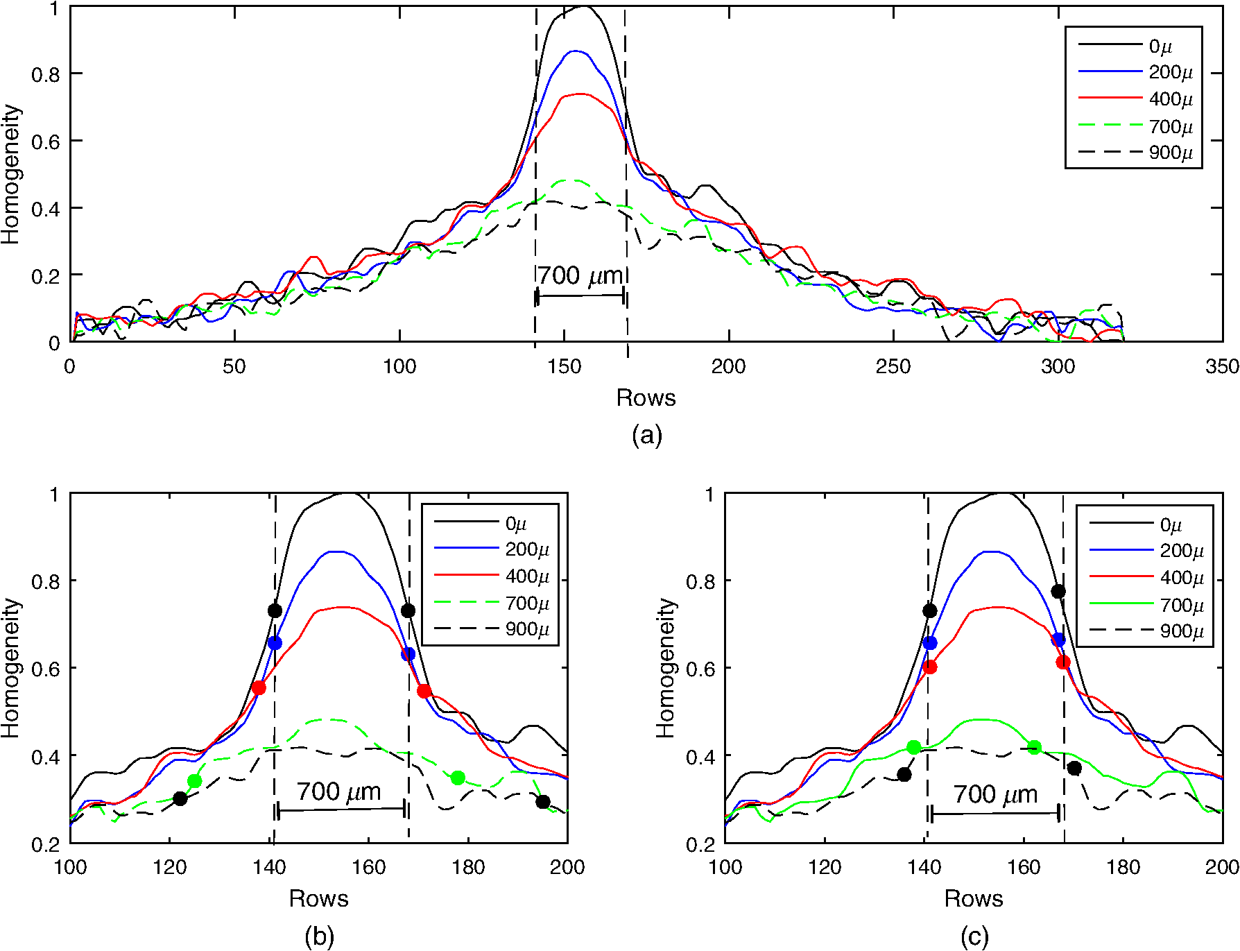 We propose a weighted standard deviation () parameter [Eq. (5)] that compensates the flattening of the distribution caused by the increasing depth. The weight () depends on the ratio between the kurtosis of the homogeneity profile at a given depth () and the kurtosis of reference . The deeper the vessel, the lower the . Thus, controls the proportion that must be considered from the standard deviation at a given depth (); therefore, it restricts the peak width associated to the vessel region. Figure 7(c) shows the vessel location obtained with , as we observe it fits best with the actual vessel location, The proposed methodology is summarized in Fig. 8, where the input is an RSI image processed by an analysis window, just as it is in a traditional LSI, in order to calculate its corresponding CM and homogeneity values. Once the homogeneity has been calculated for the whole image, the kurtosis analysis is made by sections and the blood vessel is located according to Eq. (5). Finally, a segmented image that shows only the vessel region is obtained.4.Results4.1.Linear VesselIn order to assess the proposed methodology under different conditions, we tested it using another set of RSI obtained at different depths as described in Table 2. Table 2Characteristics of the set S2 of RSI used for testing the proposed methodology.
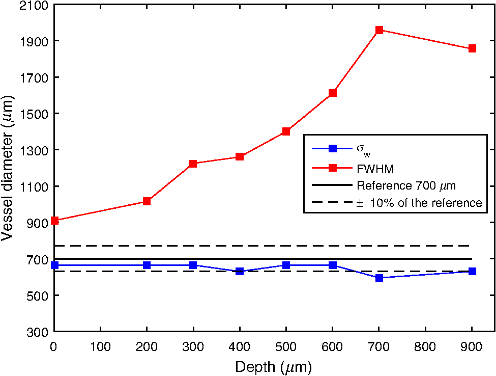
For the set S2, the vessel was manually located among the rows [141, 168] for , and this location is used as a reference for future analysis, whereas for other depths, the location of the straight vessels was done automatically by searching for the peak of the homogeneity profiles and performing the kurtosis analysis. The proposed methodology was first tested in straight vessels by processing homogeneity profiles for each column and computing the kurtosis analysis. Figure 9 shows the vessel extracted from S2 at different depths and with a velocity of . As one can see, the located vessel is better defined at lower depths. At higher depths, the image is noisier, and therefore, the homogeneity values in static and dynamic regions become similar and harder to define. Fig. 9Automatic vessel location at different depths by the proposed methodology: (a) , (b) , (c) , and (d) ; colors are related to the homogeneity values. 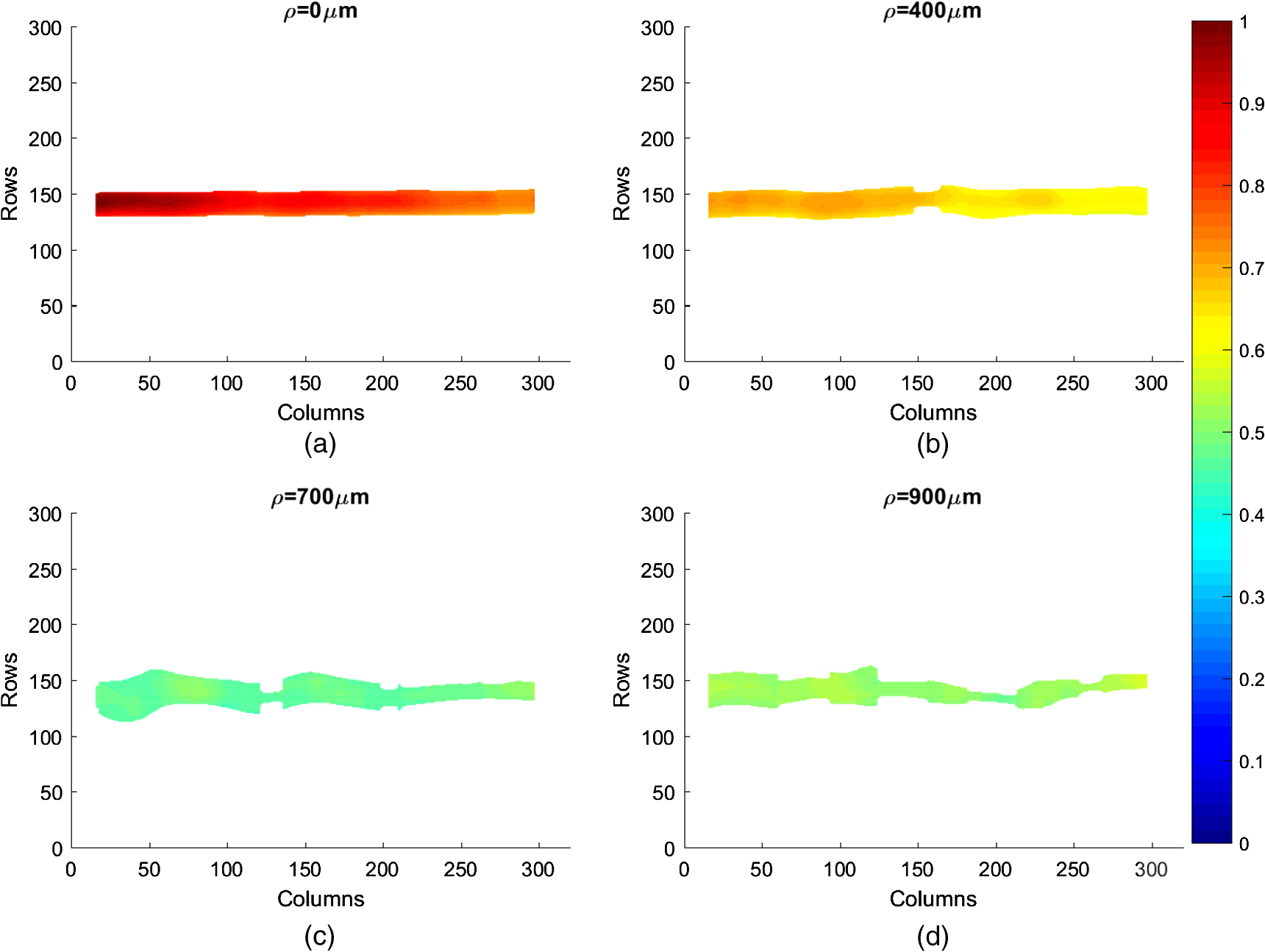 The goal of performing in vitro tests at different depths is to demonstrate that allows the estimated vessel location to match with the real vessel location, and therefore, it is possible to measure the vessel diameter. For our skin phantoms, it is a known value (). Thus, based on the obtained location at each depth, we were able to estimate the vessel diameter and its deviation from its actual value. Figure 10 shows the plot of this estimation for set S2 by comparing the results at two velocities. We can observe that the speed does not seem to affect the estimation significantly of the vessel diameter as the majority of the values lies within 10% of the actual vessel diameter (dashed lines). The plot shows how close the automatic location is to the reference diameter (solid line). 4.2.Bifurcated VesselIn in vivo situations, the vessels are not straight but takes complicated forms and even bifurcations. In order to apply our proposed kurtosis analysis, a bifurcated vessel with a diameter of and a depth of was tested [Fig. 11(b)]. In this vessel morphology, the analysis of distributions is performed along each column and each row. Fig. 11(a) Homogeneity profile for , (b) bifurcated vessel at in the RSI, (c) homogeneity profile for , and the segmentation of the bifurcated vessel according to the estimated location using kurtosis analysis over (d) a contrast and (e) a homogeneity representation.  Figure 11(a) shows the unidimensional profile corresponding to column , where the two main peaks indicate a high homogeneity area related to the left branches of the vessel [Fig. 11(b)]. The same analysis is performed but along the row [Fig. 11(c)]. It is important to remark that only the most prominent peaks are considered, and each one is analyzed as an individual distribution. Evidently, these peaks match with the center of the vessel branches but they cover a wider area than the reference as expected. For instance, the upper peak in Fig. 11(a) comprises rows [210, 270]. However, using the proposed parameter , a better location of the vessel is achieved once again now between rows [233, 251]. The final location of the vessel is given by adding both results, and it is used as a marker. When this marker overlaps with the homogeneity representation, it generates the segmented image of the vessel. Figures 11(d) and 11(e) show the result of automatic vessel location performed in the contrast and homogeneity representations. Although the vessel is well located in both representations, it presents a poorer definition in the contrast representation unlike the homogeneity representation, which retains better the vessel shape. The white lines in Fig. 11(b) indicate the ideal definition and location of the vessel. 4.3.DiscussionThe full width half maximum (FWHM) is a common measure often used to estimate the width of a function or signal.29 In this way, the FWHM and accomplish a similar function. Here, we compare the performance for vessel location of the FWHM and measurements for each depth (set S2). Figure 12 shows the differences in the vessel diameter when the vessel location is estimated with and with FWHM. We can observe that the FWHM has a marked deviation from the actual diameter, mainly for higher depths since the homogeneity profiles tend toward a normal distribution. As shown in Fig. 10, the deviation of the automatic location proposed here is smaller than the 10% (dashed lines) of the diameter of the reference (black continuous line). With the aim of measuring the error between and FWHM, the coefficient of the variation of the root-mean-square error [CV(RMSE)] was calculated by Eq. (6), where is the actual vessel diameter, is the diameter estimated for each depth, and is the mean value of the estimations. Error estimation for S2 (Fig. 12) indicates values of and . Although the main objective of this work is to locate the vessel, we were able to provide an accurate estimation of its diameter based on . Since the homogeneity provides a representation where the transitions between the static and dynamic regions are smoother, the kurtosis analysis allows locating the blood vessels accurately. Although the kurtosis analysis can also be applied to the traditional contrast representation, it provides less accurate results because of the high variations in its representation [Fig. 5(b)] as shown in Fig. 11. However, both representations can complement each other. On one hand, contrast is a well-known representation and provides information to calculate the speckle flow index (SFI), which is proportional to the blood flow velocity.30 On the other hand, the homogeneity representation and its kurtosis analysis provide a better blood vessel location even at higher depths. Therefore, the result of the latter can be used as a marker to indicate the region where the former should be calculated and still obtain the SFI.Table 3 shows a comparison among different methods based on LSI analysis to improve the visualization of deep (hundreds of microns) blood vessel. Some of them use an external agent, for example, photothermal-LSI uses a 595-nm laser pulse to thermally excite the blood flow, resulting in a local increase of temperature and thus, a transient decrease in speckle contrast;7 this technique should not be applied on temperature-sensitive areas, such as brain. PCTOC uses glycerol to reduce the scattering of in vivo and ex vivo skin samples; 60 min after the application of PCTOC, a sequence of RSI is acquired and processed with the LSI algorithm.9 LSI-SFDI uses structured illumination and LSI to separate a 2-mm-diameter shallow vessel (2 mm depth) from a deeper one (4 mm depth) but the vessel diameter is not estimated.22 Postnov et al.10 proposed an image-processing algorithm based on second-order gradient analysis of LSI images to estimate the vessel diameter and blood flow from an exposed rat mesenterium and a mouse cortex. Our results compare quite well with the previous results but, in addition, can improve the visualization of deep vessels and estimate its diameter without the use of external agents and in a noninvasive way. Table 3Reported works for visualizing deep blood vessels.
Although in all image-processing methods there is a loss of information, due to the required processes for generating the homogeneity representation and the kurtosis analysis, there is also a trade-off in the location of the blood vessel that has demonstrated to be accurate. Moreover, the homogeneity representation visually improves the blood vessel definition, and whereas the loss of information is inevitable, new information is also gained (vessel location). It is important to remark that several versions of the information are generated as the information is being processed and then, at the end of our process, the segmented image can be used as a marker. The resulting marker in our proposal can be used just for indicating the vessel location, as the white lines in Fig. 11(b), over the homogeneity representation or over the raw speckle. In this way, original and new information can be complemented. Even more, if a contrast representation is also computed, the marker can be used over it. 5.ConclusionsIn this work, it has been demonstrated that by exploring a representation based on the homogeneity values and using second-order statistics, it is possible to improve the visualization and definition of deep blood vessel regions in RSI obtained from skin phantoms. Moreover, a relationship between the vessel region and high kurtosis levels has been demonstrated. The kurtosis analysis tests prove that it is possible to obtain well-defined vessels and provide a good accurate estimation of their corresponding diameter. This work provides a methodology that works automatically and can locate vessels with different morphologies and depths as large as in depth, three times the depth previously reported by other authors. Nevertheless, it is necessary to apply the proposed methodology in in vivo experiments. This research topic will be addressed in future work. AcknowledgmentsR. Chiu would like to thank the Mexican Council of Sciences and Technology (CONACyT) for their support through grant 261148. R. Ramos-Garcia thanks the project FONCICYT/01/2016 C0013-2014-01-246648 for their financial support. E. Perez-Corona thanks the CONACyT for the scholarship 549369. ReferencesJ. D. Briers and S. Webster,
“Laser speckle contrast analysis (LASCA): a nonscanning, full-field technique for monitoring capillary blood flow,”
J. Biomed. Opt., 1
(2), 174
–179
(1996). http://dx.doi.org/10.1117/12.231359 JBOPFO 1083-3668 Google Scholar
Y. A. Aizu and T. Asakura,
“Bio-speckle phenomena and their application to the evaluation of blood flow,”
Opt. Laser Technol., 23
(4), 205
–219
(1991). http://dx.doi.org/10.1016/0030-3992(91)90085-3 Google Scholar
M. Draijer et al.,
“Review of laser speckle contrast techniques for visualizing tissue perfusion,”
Lasers Med. Sci., 24
(4), 639
–651
(2009). http://dx.doi.org/10.1007/s10103-008-0626-3 LMSCEZ 1435-604X Google Scholar
D. A. Boas and A. K. Dunn,
“Laser speckle contrast imaging in biomedical optics,”
J. Biomed. Opt., 15
(1), 011109
(2010). http://dx.doi.org/10.1117/1.3285504 JBOPFO 1083-3668 Google Scholar
P. G. Vaz et al.,
“Laser speckle imaging to monitor microvascular blood flow: a review,”
IEEE Rev. Biomed. Eng., 9 106
–120
(2016). http://dx.doi.org/10.1109/RBME.2016.2532598 Google Scholar
W. Verkruysse et al.,
“Thermal depth profiling of vascular lesions: automated regularization of reconstruction algorithms,”
Phys. Med. Biol., 53
(5), 1463
–1474
(2008). http://dx.doi.org/10.1088/0031-9155/53/5/019 PHMBA7 0031-9155 Google Scholar
C. Regan, J. C. Ramirez-San-Juan and B. Choi,
“Photothermal laser speckle imaging,”
Opt. Lett., 39
(17), 5006
–5009
(2014). http://dx.doi.org/10.1364/OL.39.005006 OPLEDP 0146-9592 Google Scholar
J. Kim, J. Oh and B. Choi,
“Magnetomotive laser speckle imaging,”
J. Biomed. Opt., 15
(1), 011110
(2010). http://dx.doi.org/10.1117/1.3285612 JBOPFO 1083-3668 Google Scholar
T. Son, J. Lee and B. Jung,
“Contrast enhancement of laser speckle contrast image in deep vasculature by reduction of tissue scattering,”
J. Opt. Soc. Korea, 17
(1), 86
–90
(2013). http://dx.doi.org/10.3807/JOSK.2013.17.1.086 1226-4776 Google Scholar
D. D. Postnov, V. V. Tuchin and O. Sosnovtseva,
“Estimation of vessel diameter and blood flow dynamics from laser speckle images,”
Biomed. Opt. Express, 7
(7), 2759
–2768
(2016). http://dx.doi.org/10.1364/BOE.7.002759 BOEICL 2156-7085 Google Scholar
N. V. Petrov, P. V. Pavlov and A. N. Malov,
“Numerical simulation of optical vortex propagation and reflection by the methods of scalar diffraction theory,”
Quantum Electron., 43
(6), 582
–587
(2013). http://dx.doi.org/10.1070/QE2013v043n06ABEH015190 QUELEZ 1063-7818 Google Scholar
T. Jeyapoovan, M. Murugan and B. C. Bovas,
“Statistical analysis of surface roughness measurements using laser speckle images,”
in World Congress on Information and Communication Technologies (WICT ’12),
378
–382
(2012). http://dx.doi.org/10.1109/WICT.2012.6409106 Google Scholar
E. R. Davies, Machine Vision: Theory, Algorithms, Practicalities, Elsevier, Amsterdam, Netherlands
(2004). Google Scholar
N. Brancati, M. Frucci and G. S. di Baja,
“Image segmentation via iterative histogram thresholding and morphological features analysis,”
in Int. Conf. Image Analysis and Recognition,
132
–141
(2008). Google Scholar
J. A. Arias-Cruz et al.,
“Visualization of deep blood vessels in speckle imaging using homogeneity measurement of the co-occurrence matrix,”
Proc. SPIE, 9660 96601O
(2015). http://dx.doi.org/10.1117/12.2196206 PSISDG 0277-786X Google Scholar
R.-S. Lu et al.,
“Grinding surface roughness measurement based on the co-occurrence matrix of speckle pattern texture,”
Appl. Opt., 45
(35), 8839
–8847
(2006). http://dx.doi.org/10.1364/AO.45.008839 APOPAI 0003-6935 Google Scholar
R. M. Haralick, K. Shanmugam and I. H. Dinstein,
“Textural features for image classification,”
IEEE Trans. Syst., Man, Cybern., SMC-3
(6), 610
–621
(1973). http://dx.doi.org/10.1109/TSMC.1973.4309314 Google Scholar
C. Palm,
“Color texture classification by integrative co-occurrence matrices,”
Pattern Recognit., 37
(5), 965
–976
(2004). http://dx.doi.org/10.1016/j.patcog.2003.09.010 PTNRA8 0031-3203 Google Scholar
X. Huang, X. Liu and L. Zhang,
“A multichannel gray level co-occurrence matrix for multi/hyperspectral image texture representation,”
Remote Sens., 6
(9), 8424
–8445
(2014). http://dx.doi.org/10.3390/rs6098424 RSEND3 Google Scholar
A. Drimbarean and P. F. Whelan,
“Experiments in colour texture analysis,”
Pattern Recognit. Lett., 22
(10), 1161
–1167
(2001). http://dx.doi.org/10.1016/S0167-8655(01)00058-7 PRLEDG 0167-8655 Google Scholar
R. B. Saager et al.,
“Multilayer silicone phantoms for the evaluation of quantitative optical techniques in skin imaging,”
Proc. SPIE, 7567 756706
(2010). http://dx.doi.org/10.1117/12.842249 PSISDG 0277-786X Google Scholar
A. Mazhar et al.,
“Laser speckle imaging in the spatial frequency domain,”
Biomed. Opt. Express, 2
(6), 1553
–1563
(2011). http://dx.doi.org/10.1364/BOE.2.001553 BOEICL 2156-7085 Google Scholar
A. B. Parthasarathy et al.,
“Robust flow measurement with multi-exposure speckle imaging,”
Opt. Express, 16 1975
–1989
(2008). http://dx.doi.org/10.1364/OE.16.001975 OPEXFF 1094-4087 Google Scholar
O. Barajas et al.,
“Monte Carlo modelling of angular radiance in tissue phantoms and human prostate: PDT light dosimetry,”
Phys. Med. Biol., 42
(9), 1675
–1687
(1997). http://dx.doi.org/10.1088/0031-9155/42/9/001 PHMBA7 0031-9155 Google Scholar
M. Klarhofer et al.,
“High-resolution blood flow velocity measurements in the human finger,”
Magn. Reson. Med., 45
(4), 716
–719
(2001). http://dx.doi.org/10.1002/mrm.1096 Google Scholar
J. Briers and A. Fercher,
“Retinal blood-flow visualization by means of laser speckle photography,”
Invest. Ophthalmol. Visual Sci., 22
(2), 255
–259
(1982). Google Scholar
W. W. Hines, D. C. Montgomery and D. M. G. C. M. Borror, Probability and Statistics in Engineering, John Wiley & Sons, Hoboken, New Jersey
(2008). Google Scholar
W. Burger et al., Principles of Digital Image Processing, Springer, New York
(2009). Google Scholar
D. L. Snyder et al.,
“Noise and edge artifacts in maximum-likelihood reconstructions for emission tomography,”
IEEE Trans. Med. Imaging, 6 228
–238
(1987). http://dx.doi.org/10.1109/TMI.1987.4307831 ITMID4 0278-0062 Google Scholar
J. C. Ramirez-San-Juan et al.,
“Impact of velocity distribution assumption on simplified laser speckle imaging equation,”
Opt. Express, 16
(5), 3197
–3203
(2008). http://dx.doi.org/10.1364/OE.16.003197 Google Scholar
BiographyHayde Peregrina-Barreto received her PhD in engineering from the Universidad Autonoma de Queretaro, Mexico, in 2011. She conducted postdoctoral research in medical imaging at the National Institute for Astrophysics, Optics, and Electronics (INAOE), Mexico, in 2014, where she is currently a full-time researcher. She has published book chapters, journals, and conferences, and is member of the Mexican National Research System (SNI). Her research interests include image processing and medical imaging. Elizabeth Perez-Corona received her bachelor’s degree in electronic engineering from Quetzalcoatl University in Irapuato, Mexico, in 2011, and received her Master of in Science degree in optics from the INAOE, Puebla, Mexico, in 2015. Currently, she is an optics PhD student at the INAOE. Her research activities are focused on biophotonics and digital image processing. Jose Rangel-Magdaleno received his PhD in engineering from the Universidad Autonoma de Queretaro, Mexico, in 2011. Currently, he is a full-time researcher at the INAOE, Mexico. He has authored one book and more than 50 works published in book chapters, journals, and conferences. He is a member of the SNI, level 1. His research interests include FPGAs, signal and image processing, instrumentation, and mechatronics. Ruben Ramos-Garcia is a senior researcher at the Optics Department of the INAOE, Puebla, Mexico, since 1997. He received his PhD at Imperial College working on photorefractive effects in crystals. His current research interests include optical tweezers, laser-induced cavitation, and photodynamic therapy. Roger Chiu received his bachelor’s degree in electronic engineering from the Instituto Tecnologico de Tuxtla Gutierrez Chiapas, master’s degree in electric engineering from the Universidad de Guanajuato, PhD in optics from the Instituto Nacional de Astrofisica, Optica y Electronica, and a postdoc in biomedical optics from Beckman Laser Institute University of California. Currently, he is a researcher at the Universidad de Guadalajara. His main research areas include biomedical optics, nonlinear optics, and optical metrology. Julio C. Ramirez-San-Juan has been a full-time researcher at the INAOE, since 2005. He received his PhD and MSc degree from the same institute, in 2003 and 1999, respectively, and his BSc degree from the Science School at the National University of Mexico. He was a postdoc at Beckman Laser Institute, University of California, Irvine, USA, from 2003 to 2005. His main research area is biophotonics. |