
|
|
1.IntroductionThe primary risk factor for glaucoma progression is intraocular pressure (IOP) that is too high.1–4 IOP represents a balance of aqueous humor production in the eye and aqueous humor outflow (AHO) through the conventional and unconventional pathways. Usually, IOP is considered to be high in glaucoma due to increased AHO resistance in the conventional outflow pathway.5 The conventional outflow pathway starts with aqueous humor flowing past the trabecular meshwork (TM), into Schlemm’s Canal (SC)6 located along the limbus, through a number of collector channels (CCs), leading ultimately to an intrascleral venous plexus, aqueous veins, and episcleral veins. Multiple reports of conventional AHO pathway structural imaging have been published. Methods have included microcomputed tomography (micro-CT) or optical coherence tomography (OCT) in both perfused postmortem eyes or live normal individuals.7–11 The advantages of postmortem eyes include the lack of shadowing from blood-filled surface vessels and avoidance of motion artifacts. An advantage of OCT is noncontact and noninvasive imaging suitable for live patients. Pilocarpine administration has been shown to influence OCT-imaged outflow structures.12–14 Automated detection of SC has also been described in rodents (Mukherjee et al. IOVS 2016; 57:ARVO E-Abstract 5936). Phase-based OCT (PhS-OCT) has shown dynamic motion in TM and post-TM outflow pathways with demonstration of a pulsatile tempo likely related to the cardiac cycle.15 Since OCT provides information in optical slices, much of the OCT work above has been based on sampled information from localized regions of the eye. Therefore, a full representation of the AHO structural framework in one eye is still required. Here we performed noninvasive imaging of AHO pathways using spectral-domain OCT, 360 deg around the limbus in one eye of a living individual. We also developed an automated detection method to identify first-order (SC and CCs) AHO structures. OCT-based definitions of CCs were proposed. Expert graders were used to validate the detection method. With an automated detection method in live humans, investigators can start to study individual variations, differences between two eyes of one individual, and diseased versus normal eyes. With this information, ophthalmologists may be able to target surgeries for optimal IOP-lowering results. 2.Methods2.1.Test SubjectThe right eye of a 35-year-old healthy Middle Eastern male with no medical history or ocular history was used for this study. This study was approved by the Institutional Review Board of UCLA and performed in accordance with the tenets of the Declaration of Helsinki. Written informed consent was obtained. The subject had a best-corrected visual acuity of 20/20 with a refraction of . The patient had no family history of glaucoma or personal history of ocular hypertension. The exam was only notable for a small nasal pinguecula. 2.2.Image AcquisitionAnterior segment SD-OCT imaging was performed with the Heidelberg Spectralis (Heidelberg Engineering, Germany) using the anterior segment lens/module on scleral mode with oversampling (automated real-time = 9) and TruTrak tracking (Fig. 1). Topical proparacaine was given to the eye. Five overlapping scans were taken from each of the eight cardinal positions (superior, superior-temporal, temporal, inferior-temporal, inferior, inferior-nasal, nasal, and superior nasal). Temporal and nasal volumes utilized horizontal scans. Superior and inferior volumes utilized vertical scans. All other positions were oblique. Using a Heidelberg Engineering developed custom script for decreased B-scan to B-scan distance, each volume scan was composed of 128 B-scans over a scan angle for final axial/lateral/B–B scan resolution of , respectively. While tracking was indispensable to counteract motion artifact, slow volume acquisition required 1 to 2 min of time per volume. The subject experienced dry eye discomfort. To minimize the risk of corneal damage, artificial tears were applied with substantial rest periods in between image acquisition sessions. As CCs are small (),6 the decreased B-scan to B-scan distance was important to limit missing them. However, this meant a large number of B-scans was needed to cover the limbus circumferentially. In the end, we obtained 40 volumes totaling a substantial number of B-scans for one subject (#5114). 2.3.Image ProcessingFocused on analyzing this large batch of data from one eye, three-dimensional (3-D) SD-OCT images were exported to a numerical computing language (MATLAB; MathWorks, Natick, Massachusetts). SC was defined as an OCT-signal hypodense (low-reflective) structure in the perilimbal region near the angle. Due to inconsistent angle location in each OCT B-scan across the eye and variable image quality, automated detection of outflow pathways based solely on the OCT images was challenging. To overcome this problem, we proposed a hierarchical method for SC and CC detection and segmentation. The image acquisition device provided the B-scan in addition to the confocal scanning laser ophthalmoscopic (CSLO) image, which corresponded to each rectangle (Fig. 1). Therefore, the CSLO images were used as a first step to approximate the location of the angle to initiate SC detection. Using a Bayesian ridge approach,16 the scleral-cornea border was identified in this region to (1) approximate the angle’s location in the OCT images and (2) to account for the curvature around the limbus. Then, a crossmultiplication method was used to relocate the delineated curvature for the OCT images. For example, if the ridge was in the middle of the CSLO images, the approximate location of the angle would be in the middle of the OCT B-scan image. This estimated area was used as a starting point to segment both SC and CC. Then, a fuzzy hidden Markov chain algorithm was used to segment both SC and CC. Fuzzy hidden Markov model-based automatic segmentation algorithms allow noise modeling and have proven to be less sensitive to ambiguous tissue borders than other segmentation approaches.17 These algorithms offer an unsupervised estimation of the parameters needed for the image segmentation and limit the user’s input to the number of classes to be searched for in the image.17 In particular, we have defined four classes: (1) the SC, (2) the CC, (3) the anterior segment tissue, and (4) the noise (i.e., area of the image that does not correspond to the anterior segment). Each class was modeled with a gamma distribution with different values of hyper-parameters ( and ), where . To refine the segmentation of the CC, we defined the following parameters. First, CCs were defined as OCT-signal hypodense (low-reflective) structures that, when emanating from the posterior tip of SC, had an angle theta of 15 deg to 170 deg (Fig. 2). Second, if not from the posterior tip of SC, CCs could only arise from the dorsal portion of the posterior 50% of the SC with an angle theta of 15 deg to 115 deg (Fig. 2). The first criterion acknowledged that there would be no way for a method to distinguish a CC that emanated in-line from the posterior tip of SC from an unusually long SC. The second criterion acknowledged an arc-like hyporeflective band oft-seen in anterior segment OCT.9 Current literature labels this structure as the TM-interface band although no exhaustive ground-truth OCT:histological study has proven its identity. Nevertheless, the position of this band is superior to the scleral spur and inferior to Schwalbe’s line, suggesting that this structure may be TM-related. Given its low OCT reflective status, we found that automated detection methods designed to find low-reflective structures could identify this band and confuse it for CCs. Therefore, while unclear if this structure truly represents outflow lumens or not, we decided to remain consistent with current conventions by excluding it in automated detection. Fig. 2Definition of collector channels. (a) A hyporeflective band (interphase shadow) is seen on anterior segment OCT that is believed to be the trabecular meshwork.9 (b) Given its OCT low reflectivity status, it can be confused for aqueous humor outflow pathway lumens on automated segmentation as an anterior pointing collector channel (CC). Therefore, CCs were defined as, if arising from the dorsal portion of SC, arising only on the dorsal 50% of SC and with an angle of 15 to 115 deg to avoid the hyporeflective band. Also, an angle of 15 to 170 deg was acceptable if CC arose from the posterior tip of Schlemm’s canal (SC) because CC arising in-line from the posterior tip of SC could not be distinguished from an extra-long SC.  2.4.Expert GradingThe expert graders (AD and AH) used were accustomed to reading OCT as a part of routine clinical care, have been involved in the past with clinical trials utilizing anterior segment imaging, and were the team members that developed the above definitions for automated detection of AHO pathways. In an iterative process, definitions would be made, automated detection was applied, and graders would observe the results with subsequent adjustment to the definition until the final criteria were settled upon as above. To assess the accuracy of the automated detection method, specific questions were applied to two-dimensional (2-D) B-scan results. First, each B-scan was graded for image quality as either gradable (visible cornea, sclera, iris, and angle recess without excessive shadowing) or ungradable. The automated detection of each B-scan was then graded in a masked fashion using six questions with an answer of “yes” or “no.” The following grading questions were applied to every single B-scan obtained.
The results from both graders were tabulated into a table format (Tables 1Table 2Table 3Table 4Table 5–6), and Cohen’s kappa coefficients were calculated to determine intergrader agreement (Table 7). Separately, as not every single B-scan had a CC, assessing for false-negative detection using a denominator of total graded B-scans () would artificially improve the accuracy of the automated detection method. Therefore, true false negatives were assessed dividing the total agreed false negatives ( in Table 5) by the total number of B-scans with observed CC (). Statistical analysis was performed using SPSS version 18.0 (SPSS Inc., Armonk, New York). Table 1Was SC missed by automated detection?
% “No” by both graders = 98.3% Table 2Was SC falsely identified by automated detection?
% “No” by both graders = >99.9% Table 3Was SC underestimated by automated detection?
% “No” by both graders = 94.9% Table 4Was SC exaggerated by automated detection?
% “No” by both graders = >99.9% Table 5Were CC completely missed by automated detection?
% “No” by both graders = 94.3% Table 6Were CC falsely identified by automated detection?
% “No” by both graders = 98.6% Table 7Agreement in grading between the two graders.
2.5.Three-Dimensional ReconstructionTo reconstruct the 360-deg 3-D representation of SC and CCs from OCT B-scans, the CSLO image was used to stitch together the different volumes. When two or more volumes overlapped in one area, the mean of the SC and CC was calculated. Hence, the B-scans were aligned in 3-D space, using the infrared image associated with each OCT B-scan as a girdle framework. This averaging in overlap regions helped overcome parallax errors from imaging from different perspectives and distortions at edges of volumes. The number of total unique CCs was counted, given the following criteria: (1) the collector should be present in every overlapped volume, (2) the length of each collector should have at least five connected pixels, and (3) each collector should be present in at least 10 consecutive B-scans. This final 3-D reconstruction was then opened in Imaris (7.3.0; Bitplane, Zurich, Switzerland) for isosurface mapping and polygonal reconstruction for SC and CCs.18,19 3.ResultsThe automated detection method qualitatively identified SC and CC (Figs. 3 and 4). Even septa within the SC could be distinguished [Figs. 3(c) and 3(d)]. As described in the methods, anterior segment OCT literature acknowledges the presence of an arc-like low OCT-reflectivity hypodensity for which the convention is to identify as being TM-related (Figs. 2 and 5). To remain consistent with this convention, we designed the automated detection method to avoid this structure (Fig. 5). Fig. 3Automated detection of SC. (a) SC is clearly seen (yellow arrow) with (b) good identification. (c) In one case, a small septum (yellow arrowhead) splits the SC (yellow arrow). (d) This septum is recognized and avoided by the detection method.  Fig. 4Automated detection of CC. (a) SC is clearly seen without a CC directly attached to the posterior tip of SC. (b) Therefore, only SC is detected. (c) In a case of a clear CC (yellow arrowhead) arising from the posterior tip of SC (yellow arrow). (d) The CC is additionally identified.  Fig. 5Avoidance of the TM hyporeflective band. (a) An OCT hyporeflective shadow (yellow arrowhead) that is often attributed to the TM is seen. This can appear to be attached to the anterior and dorsal portion of SC (yellow arrow). (b) While unclear in its origin, to stay in convention with the literature, CC was defined to avoid this structure. 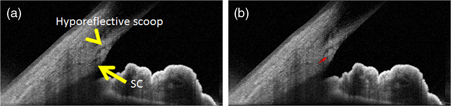 To test the accuracy and precision of this method, expert readers were used. Only 48 out of 5114 (0.009%) images were determined to be ungradable. The predominant reason for ungradable images was surface vessel or structure-related (pinguecula) shadowing. A series of questions (see Sec. 2) to validate the automated detection method was posed for every single B-scan. tables for two graders are shown (Tables 1–6). Most importantly, the method performed well; the two graders agreed that errors were made (answer of “yes” by each grader) only to 5.7% of the time. Stated in reverse (“no” by each grader), the two graders agreed that 98.3%, 94.9%, , and of the time SC was not missed, underestimated, falsely identified, or exaggerated, respectively. Kappa values for questions 1 to 6 were good, ranging from 0.63 to 0.78 (Table 7), except for the case of question 4 (exaggerated SC detection), where the kappa was low (0.16, Table 7). Here, the overall incidence of exaggerated SC detection by the automated software was also extremely low (Table 4), which can directly lead to a small kappa value. For CCs, since not every B-scan showed a CC, the tables were appropriate for assessing agreement between the graders but may have exaggerated how well the method performed. Therefore, to determine true false negatives, the total number of false negatives was divided by the total number of B-scans with CCs () as opposed to the total number of graded B-scans. During image acquisition, because a single and distinct CC could be seen on multiple B-scans, the total number of B-scans with a CC did not equal the total number of CCs. Also, since B-scans overlapped (Fig. 1), one unique CC could be represented more than once on separate volumes. Therefore, to count the total number of CCs, distinct CCs were defined as positive identification (see CC criteria in methods) that was found in at least 10 consecutive B-scans and that was represented in both volumes if the CC was located in a region found in two separate overlapping volumes. Based on this, a total of 24 CCs were counted when including CC of at least 5 pixels in length. Changing the number of consecutive B-scans () did not affect the results. Varying the length of the CCs up to 8 pixels did not change the results, but at 9 pixels the number of collectors did decrease to 18. 2-D B-scans were then organized into a 3-D caste of AHO pathways [Figs. 6(a) and 6(b)]. Segmental anatomy was seen with certain areas showing wider or narrower SC [Fig. 6(c)]. CCs [Fig. 6(d)] could be distinguished as well. Fig. 63-D construction of AHO pathways. (a) B-scans were arranged in 3-D space using the CSLO image as a framework for isosurface mapping in an Apple-Miyake view. (b) External view. (c) Different areas of SC can appear thinner or wider (blue arrows). (d) First-order CC roots are seen (green arrows).  4.DiscussionHere we report the development of an automated AHO detection method with the highest available resolution ( B-scan to B-scan; most commercial devices have a B-scan to B-scan distance) aimed at identifying SC and prominent first-order CCs in the intact eye of a living individual. With any detection method, the final result is only as good as the detection criteria and philosophy on which the method is based. Here, our goal was a detection method that (a) did not create false structures and (b) if in error would err on the side of missing smaller structures. We feel that we have accomplished this by very low false-positive detection rates and low but still present false-negative detection rates. When converted into a 3-D construct, one clearly sees variability in SC size with identifiable CCs. The automated detection method was precise. Good reproducibility between expert readers was seen in the tables with good Cohen’s kappa values. Both graders also agreed that the automated detection method was accurate, especially for SC (98.3%). Cohen’s kappa is generally considered a more robust test compared with percent agreement, given that it controls for the agreement that might occur simply by chance.20 However, it must be noted that kappa values are known to be flawed in circumstances of low incidence.21 The remarkably low incidence (Table 4) of exaggerated SC detection, therefore, explains its low kappa value (0.159). In all cases, presenting the data as tables transparently showed the raw values. Also, while detection of SC was robust, the identification of CCs was inherently more challenging for several reasons that may have led to increased false negatives (at least ) or an underestimate of the total number. First, we stopped our detection at first-order CCs that were in direct communication with SC. The reason for this was because this detection method was aimed at OCT low-reflective structures. In the sclera, other anterior segment OCT low-reflective lumens not associated with AHO exist (arteries, veins, and lymphatics). Therefore, expanding the automated detection method for lumens not in direct contact with SC and posterior to the perilimbal area would have created a complicated segmentation result including both AHO- and non-AHO related structures. Second, to distinguish true CCs from (a) an extra-long SC or (b) from the TM interphase shadow, definitions of CCs had to be created (see Sec. 2). Recent CC research with scanning electron microscopy has recognized that CC can take on simple configurations with a circular orifice or complex CC configurations with flaps or tortuous CC/SC connections.11 Due to this, we likely missed CCs in-line from SC, CCs that may have arisen from the anterior/dorsal portions of SC close to the TM interphase shadow, or tortuous CCs emanating out of plane from SC on the B-scan. Third, despite good resolution, small CCs could fall between B-scans, or two CCs close in space may not have been resolved as being separate. Fourth, based on a philosophy driven by prioritizing a very low false-positive detection rate at the risk of possible false-negative detection, small single CCs or signal-fuzzy CCs on B-scans located at the edges of larger CCs may have been missed. Further complicating CC identification, CC biology is becoming better understood with even a dynamic component appreciated involving changes to the CC number or size under different biological conditions such as varying IOP.6 Therefore, while observing a similar number of CCs to previously published literature (24 to 37 CCs in normal eyes), this method had increased false negatives with a possible underestimate in the total number.6,22,23 In the end, this method may be more suited for detecting SC and roots of bigger and classical CCs. Special consideration should also be made for the arc-like TM interphase shadow near SC commonly seen on anterior segment OCT (Fig. 2).9 As the arc-like interphase shadow showed low reflectivity, it was easily confused for an AHO lumen and incorporated as CCs in early builds of the segmentation method. Therefore, the CC definition was adjusted, and we excluded the interphase shadow (Fig. 5). Nevertheless, the actual identification of the interphase shadow has not been proven. In the retina, careful OCT and histology ground-truth-based image comparison led to a relabeling of the “IS-OS junction” to the “ellipsoid layer.”24,25 This showed that identifying the anatomical counterpart of an OCT-based landmark is not always easy and open to modification. Similar work needs to be done for the anterior segment. One possible approach may be to thread SC with a suture (similar to a clinical canaloplasty surgery) such that the suture serves as a fiducial/reference point for multimodal comparison between histology and OCT. Nylon sutures are known to be autofluorescent and could be identified by fluorescent microscopy.26 Finally, some limitations of this method must be discussed. While SD-OCT is noted to be very fast, volume scans with high resolution required many images. Motion tracking was crucial to counteract motion artifacts, which increased the time necessary to image 360 deg around the eye. Therefore, it took two days for circumferential imaging using volume scans, which is not compatible for everyday clinical use. This is why we focused on obtaining and analyzing a large number of B-scans (#5114) in one individual as opposed to scanning multiple subjects. Additional advances in anterior segment OCT, such as increased speed or resolution will be necessary to make anterior segment AHO pathway imaging practical enough for everyday clinical care. More specifically, we speculate that axial orientation with simultaneous image acquisition of both angles might simplify the procedure by allowing the patient to just look straight ahead without moving their eyes. Also, this will require less time as two angles are imaged at once. Longer-wavelength OCT (swept source) may also give better results with increased depth of imaging at the risk of lesser resolution. Further testing should be done in glaucomatous eyes because disease conditions make image acquisition less optimal and image processing and segmentation more difficult. In conclusion, circumferential imaging with automated segmentation and 3-D reconstruction of an intact eye in one live individual’s AHO pathways was successfully performed. Conventional AHO flows through SC, which lies along the limbus, thus creating the impression that there is uniform 360 deg outflow that radiates away from the limbus. However, substantial literature suggests that outflow is segmental instead of uniform.27–31 Real-time visualization of angiographic flow using aqueous angiography has shown this nonuniformity.32–37 Circumferential OCT imaging here confirmed a segmental structural characteristic. This result is supported by prior OCT data from sampled portions of the eye from living individuals showing pronounced segmental anatomy.10 While interesting, the underlying meaning of AHO structure on OCT is unclear. Regarding flow, a large lumen might mean decreased resistance with increased flow. Alternatively, a large lumen could also represent a stagnant pocket of trapped and unmoving fluid. Clinically, this may be important to distinguish in the future because of trabecular-targeted minimally invasive glaucoma surgeries (MIGS). Near universal placement in the nasal quadrant of the eye in the setting of segmental outflow may explain the variable success of MIGS. Therefore, improved AHO understanding with a noncontact and noninvasive modality such as anterior segment OCT may allow for customized glaucoma surgeries and better IOP lowering in the future. DisclosuresA.S.H. discloses that Heidelberg Engineering provided a custom script for decreased B-scan to B-scan distance (improved resolution) for this project. A.S.H. also receives research support from Allergan and Glaukos Corporation for research unrelated to this work. R.N.W. and L.M.Z. disclose research equipment from Heidelberg Engineering, Carl Zeiss Meditec, Topcon Inc., and Optovue Inc. The remaining authors have no conflicts of interest, financial or otherwise, to declare. AcknowledgmentsThe authors would like to thank Dr. Yohko Murakami, Dr. Chris Bowd, and Dr. Siamak Yousefi for early discussion in this project. Funding for this work was provided by the National Institutes of Health, Bethesda, Maryland [K08EY024674 (A.S.H.)] P30EY022589 (L.M.Z.), American Glaucoma Society (AGS) Mentoring for Physician Scientists Award 2013 (A.S.H.) and 2014 (A.S.H.); AGS Young Clinician Scientist Award 2015 (A.S.H.); Research to Prevent Blindness Career Development Award 2016 (A.S.H.); and an unrestricted grant from Research to Prevent Blindness (New York, New York). The funders had no role in study design, data collection and analysis, decision to publish, or preparation of the paper. ReferencesM. O. Gordon et al.,
“The ocular hypertension treatment study: baseline factors that predict the onset of primary open-angle glaucoma,”
Arch Ophthalmol., 120 714
–720
(2002). http://dx.doi.org/10.1001/archopht.120.6.714 Google Scholar
“The advanced glaucoma intervention study (AGIS): 7. the relationship between control of intraocular pressure and visual field deterioration,”
Am. J. Ophthalmol., 130 429
–440
(2000). http://dx.doi.org/10.1016/S0002-9394(00)00538-9 Google Scholar
A. Heijl et al.,
“Reduction of intraocular pressure and glaucoma progression: results from the early manifest glaucoma trial,”
Arch Ophthalmol., 120 1268
–1279
(2002). http://dx.doi.org/10.1001/archopht.120.10.1268 Google Scholar
P. R. Lichter et al.,
“Interim clinical outcomes in the collaborative initial glaucoma treatment study comparing initial treatment randomized to medications or surgery,”
Ophthalmology, 108 1943
–1953
(2001). http://dx.doi.org/10.1016/S0161-6420(01)00873-9 OPANEW 0743-751X Google Scholar
W. M. Grant,
“Clinical measurements of aqueous outflow,”
AMA Arch. Ophthalmol., 46 113
–131
(1951). http://dx.doi.org/10.1001/archopht.1951.01700020119001 Google Scholar
C. R. Hann et al.,
“Anatomic changes in Schlemm’s canal and collector channels in normal and primary open-angle glaucoma eyes using low and high perfusion pressures,”
Invest. Ophthalmol. Vis. Sci., 55 5834
–5841
(2014). http://dx.doi.org/10.1167/iovs.14-14128 Google Scholar
C. R. Hann et al.,
“Imaging the aqueous humor outflow pathway in human eyes by three-dimensional micro-computed tomography (3D micro-CT),”
Exp. Eye Res., 92 104
–111
(2011). http://dx.doi.org/10.1016/j.exer.2010.12.010 Google Scholar
T. Usui et al.,
“Identification of Schlemm’s canal and its surrounding tissues by anterior segment Fourier domain optical coherence tomography,”
Invest. Ophthalmol. Vis. Sci., 52 6934
–6939
(2011). http://dx.doi.org/10.1167/iovs.10-7009 Google Scholar
L. Kagemann et al.,
“Identification and assessment of Schlemm’s canal by spectral-domain optical coherence tomography,”
Invest. Ophthalmol. Vis. Sci., 51 4054
–4059
(2010). http://dx.doi.org/10.1167/iovs.09-4559 Google Scholar
L. Kagemann et al.,
“Visualization of the conventional outflow pathway in the living human eye,”
Ophthalmology, 119 1563
–1568
(2012). http://dx.doi.org/10.1016/j.ophtha.2012.02.032 OPANEW 0743-751X Google Scholar
M. D. Bentley, C. R. Hann and M. P. Fautsch,
“Anatomical variation of human collector channel orifices,”
Invest. Ophthalmol. Vis. Sci., 57 1153
–1159
(2016). http://dx.doi.org/10.1167/iovs.15-17753 Google Scholar
G. Li et al.,
“Pilocarpine-induced dilation of Schlemm’s canal and prevention of lumen collapse at elevated intraocular pressures in living mice visualized by OCT,”
Invest. Ophthalmol. Vis. Sci., 55 3737
–3746
(2014). http://dx.doi.org/10.1167/iovs.13-13700 Google Scholar
A. Skaat et al.,
“Effect of pilocarpine hydrochloride on the Schlemm canal in healthy eyes and eyes with open-angle glaucoma,”
JAMA Ophthalmol., 134
(9), 976
–981
(2016). http://dx.doi.org/10.1001/jamaophthalmol.2016.1881 Google Scholar
J. Chen et al.,
“Expansion of Schlemm’s canal by travoprost in healthy subjects determined by Fourier-domain optical coherence tomography,”
Invest. Ophthalmol. Vis. Sci., 54 1127
–1134
(2013). http://dx.doi.org/10.1167/iovs.12-10396 Google Scholar
P. Li et al.,
“Pulsatile motion of the trabecular meshwork in healthy human subjects quantified by phase-sensitive optical coherence tomography,”
Biomed. Opt. Express, 4 2051
–2065
(2013). http://dx.doi.org/10.1364/BOE.4.002051 Google Scholar
J. Papari et al.,
“A biologically motivated multiresolution approach to contour detection,”
EURASIP J. Adv. Sig. Process., 2007 071828
(2007). http://dx.doi.org/10.1155/2007/71828 Google Scholar
M. Hatt et al.,
“Fuzzy hidden Markov chains segmentation for volume determination and quantitation in PET,”
Phys. Med. Biol., 52 3467
–3491
(2007). http://dx.doi.org/10.1088/0031-9155/52/12/010 PHMBA7 0031-9155 Google Scholar
J. M. Gonzalez et al.,
“Tissue-based multiphoton analysis of actomyosin and structural responses in human trabecular meshwork,”
Sci. Rep., 6 21315
(2016). http://dx.doi.org/10.1038/srep21315 SRCEC3 2045-2322 Google Scholar
J. M. Gonzalez and J. C. H. Tan,
“Semi-automated vitality analysis of human trabecular meshwork,”
IntraVital, 2 e27390
(2013). http://dx.doi.org/10.4161/intv.27390 Google Scholar
J. Sim and C. C. Wright,
“The kappa statistic in reliability studies: use, interpretation, and sample size requirements,”
Phys. Ther., 85
(3), 257
–268
(2005). http://dx.doi.org/10.1093/ptj/85.3.257 Google Scholar
K. Gwet,
“Inter-rater reliability: dependency on trait prevalence and marginal homogeneity,”
Stat. Methods Inter-Rater Reliab. Assess., 2 1
–10
(2002). Google Scholar
G. Dvorak-Theobald,
“Further studies on the canal of Schlemm; its anastomoses and anatomic relations Georgiana,”
Am. J. Ophthalmol., 39
(4), 65
–89
(1955). http://dx.doi.org/10.1016/0002-9394(55)90154-9 Google Scholar
N. Ashton,
“Anatomical study of Schlemm’s canal and aqueous veins by means of neoprene casts. Part I. Aqueous veins,”
Br. J. Ophthalmol., 35
(5), 291
–303
(1951). http://dx.doi.org/10.1136/bjo.35.5.291 BJOPAL 0007-1161 Google Scholar
R. W. Lu et al.,
“Investigation of the hyper-reflective inner/outer segment band in optical coherence tomography of living frog retina,”
J. Biomed. Opt., 17 060504
(2012). http://dx.doi.org/10.1117/1.JBO.17.6.060504 JBOPFO 1083-3668 Google Scholar
R. F. Spaide and C. A. Curcio,
“Anatomical correlates to the bands seen in the outer retina by optical coherence tomography: literature review and model,”
Retina, 31 1609
–1619
(2011). http://dx.doi.org/10.1097/IAE.0b013e3182247535 RETIDX 0275-004X Google Scholar
J. C. Tan et al.,
“In situ autofluorescence visualization of human trabecular meshwork structure,”
Invest. Ophthalmol. Vis. Sci., 53 2080
–2088
(2012). http://dx.doi.org/10.1167/iovs.11-8141 Google Scholar
S. A. Battista et al.,
“Reduction of the available area for aqueous humor outflow and increase in meshwork herniations into collector channels following acute IOP elevation in bovine eyes,”
Invest. Ophthalmol. Vis. Sci., 49 5346
–5346
(2008). http://dx.doi.org/10.1167/iovs.08-1707 Google Scholar
E. D. Cha et al.,
“Variations in active outflow along the trabecular outflow pathway,”
Exp. Eye Res., 146 354
–360
(2016). http://dx.doi.org/10.1016/j.exer.2016.01.008 Google Scholar
J. Y. Chang et al.,
“Multi-scale analysis of segmental outflow patterns in human trabecular meshwork with changing intraocular pressure,”
J. Ocul. Pharmacol. Ther., 30 213
–223
(2014). http://dx.doi.org/10.1089/jop.2013.0182 Google Scholar
K. E. Keller et al.,
“Segmental versican expression in the trabecular meshwork and involvement in outflow facility,”
Invest. Ophthalmol. Vis. Sci., 52 5049
–5057
(2011). http://dx.doi.org/10.1167/iovs.10-6948 Google Scholar
J. A. Vranka et al.,
“Mapping molecular differences and extracellular matrix gene expression in segmental outflow pathways of the human ocular trabecular meshwork,”
PLoS One, 10 e0122483
(2015). http://dx.doi.org/10.1371/journal.pone.0122483 POLNCL 1932-6203 Google Scholar
A. S. Huang et al.,
“Aqueous angiography-mediated guidance of trabecular bypass improves angiographic outflow in human enucleated eyes,”
Invest. Ophthalmol. Vis. Sci., 57 4558
–4565
(2016). http://dx.doi.org/10.1167/iovs.16-19644 Google Scholar
S. Saraswathy et al.,
“Aqueous angiography: real-time and physiologic aqueous humor outflow imaging,”
PLoS One, 11 e0147176
(2016). http://dx.doi.org/10.1371/journal.pone.0147176 POLNCL 1932-6203 Google Scholar
A. S. Huang et al.,
“Aqueous angiography with fluorescein and indocyanine green in Bovine eyes,”
Transl. Vis. Sci. Technol., 5
(6), 5
(2016). http://dx.doi.org/10.1167/tvst.5.6.5 Google Scholar
A. S. Huang, C. Mohindroo and R. N. Weinreb,
“Aqueous humor outflow structure and function imaging at the bench and bedside: a review,”
J. Clin. Exp. Ophthalmol., 7 578
(2016). http://dx.doi.org/10.4172/2155-9570.1000578 Google Scholar
A. S. Huang et al.,
“Aqueous angiography in living nonhuman primates shows segmental, pulsatile, and dynamic angiographic aqueous humor outflow,”
Ophthalmology, 124 793
–803
(2017). http://dx.doi.org/10.1016/j.ophtha.2017.01.030 OPANEW 0743-751X Google Scholar
A. S. Huang et al.,
“Aqueous angiography: aqueous humor outflow imaging in live human subjects,”
Ophthalmology,
(2017). http://dx.doi.org/10.1016/j.ophtha.2017.03.058 Google Scholar
|
||||||||||||||||||||||||||||||||||||||||||||||||||||||||||||||||||||||||||||||||||||||||||||


