1.

Introduction

Photothermal (PT) imaging (PTI) of gold nanoparticles (AuNPs) has been developed as a molecular specificity approach for biomedical imaging in particular over the past decade.^1–11 In PTI, AuNPs are first biofunctionalized to bind to specific targets, e.g., antigens on biological cells membranes and then excited optically for selective imaging. The PT effect is based on the transformation of light energy into heat. Under optical excitation with specific wavelength, AuNPs can form localized plasmonic resonance (LPR), an oscillation of the electron cloud around the particle at a resonance frequency.⁵ Depending on the size and shape of the nanoparticle, this frequency may be easily engineered to vary within the entire visible spectrum and into the mid-IR region, creating a narrow absorption spectrum. Thus, when illuminating the AuNPs with a wavelength that suits their plasmonic resonance, a strong absorption of light occurs and is followed by an energy release in the form of heat. This heat creates environmental effects, such as local refractive index changes that can be detected optically. It should be noted that under sufficiently high excitation intensities, AuNPs heating may cause structural damage to their surroundings.

In order to avoid temperature buildup, time-modulated pulsed excitation is used in PTI, where the excitation frequency can change from several Hz to MHz. For this reason, PTI is not suitable for highly dynamic cells in flow, for which the dynamics frequency range overlaps with the excitation temporal frequency.⁹ Thus, the motivation for increasing data acquisition and processing rate of PTI is clear. Fast PTI will allow a significant increase of throughput suitable for flow cytometry so PTI may become a common diagnostic tool, rather than limited to research.

Interferometric phase acquisition methods, such as differential interference contrast,¹ optical coherence tomography (OCT),^2,6,7 and digital holographic microscopy (DHM),^9,11,12 are all capable of detecting optical phase changes induced by refractive index variations due to the temperature rise in the medium surrounding the heated AuNPs. OCT-based PTI has produced the best results so far, in terms of signal-to-noise ratio (SNR). However, OCT imaging is typically based on either scanning point-detection schemes or scanning line illumination, where both require costly equipment, especially when PTI of dynamic objects is needed.

In general, PTI techniques depending on scanning to obtain the full field of view (FOV) hold little potential in cost-effective imaging of dynamic objects. Moreover, in cases where the optically heated AuNPs change their position in the FOV during PTI, smeared images are formed, which affects visualization capabilities. In addition to the observation of cells during flow, the expansion of nonscanning PTI methods for usage with dynamic samples can be essential for capturing movements of tagged cellular organelles, tissue displacements, and thus, prospects to address applications which are currently hard to access by scanning-based PTI. We have recently proposed different methods for wide-field, scan-free PTI, based on our DHM systems.^9,11 Since a large region of interest (ROI) is imaged by a single camera exposure, we are also able to image highly dynamic biological samples.^13,14

Flow cytometry is a well-established method for high-throughput measurements and sorting of flowing biological cells, typically utilizing molecular specificity obtained by fluorescent biomarkers. To obtain high throughput, large amounts of cells flow through the device to produce large databases per sample in a short time. Imaging flow cytometry sacrifices throughput and cell flow velocity for better image quality and spatial data.^15,16 For this goal, AuNPs hold a significant advantage over fluorescent biomarkers, which tend to photobleach, followed by signal degradation over time.¹⁷ AuNPs do not lose their efficiency before reaching significantly high excitation powers, and PTI keeps the same SNR during long courses of time. Moreover, AuNPs heating makes them attractive as specific bioagents for heating therapy.

Over the past decades, with the development of high-speed cameras, several methods for imaging dynamic cells have been developed. Some of them involve spectrally coded imaging¹⁸ and focus-stacking phase imaging.¹⁹ These methods use high frame-rate sensors of over 3000 frames per second and may capture from tens to thousands of cells per second, flowing at a speed of between 10 and $40\mathrm{mm}/\mathrm{s}$, significantly lower than flow cytometry but in the physiological range of blood flow.²⁰

In this paper, we propose a simplified implementation of PTI for imaging cells in flow and new image processing principles for improved computational efficiency, with the potential for future integration in imaging flow cytometers. The new PTI processing approach increases the computation speed by decreasing the window size of the spectral analysis and a combination of the Goertzel discrete Fourier transform (DFT) with sliding DFT algorithms.²¹ Both approaches significantly increase the potential of PTI-based real-time imaging flow cytometry.

2.

Methods

2.1.

Optical Setup

For recording digital off-axis image holograms, we use a simplified interferometer²² that is illuminated by a low-temporal-coherence source. As shown in Fig. 1(a), our imaging beam is originated from a titanium:sapphire laser (Coherent, Micra-5, ${\lambda }_0=780\mathrm{nm}$, $\mathrm{\Delta }{\lambda }_{\mathrm{FWHM}}=10\mathrm{nm}$, up to $100\mathrm{mW}/{\mathrm{cm}}^2$, at the maximum imaging speed). The sample is illuminated by the condenser lens L1 ($f=300\mathrm{mm}$). The light that is transmitted by the sample is then magnified by a microscope objective ($40\times$, $\mathrm{NA}=0.65$, Newport), passes the tube lens L2 ($f=150\mathrm{mm}$), and enters the self-interference module.¹⁶ This module interferes the image of the sample beam with its slightly shifted version to obtain an off-axis angle between the interfering beams, which is achieved by a slight tilt of one of the mirrors, so that the sample details in one beam overlap with empty locations in the shifted beam. The resulting interferograms are recorded by a CCD camera. Here, we choose to work with a resolution of $2\mu \mathrm{m}$, which is enough to acquire PT signals from the cells, in order to image a large FOV. Note that our goal here is not to see the binding sites of the AuNPs on the cells but rather just to obtain PT from the labeled cells during fast flow.

Fig. 1

Sample setup for dynamic PTI of cells in flow. (a) The PTI system, comprised of a simplified interferometric setup (red beams) and PT setup (green beam). In the interferometric path, a titanium:sapphire (Ti:sapph) laser beam is condensed by lens L1 and imaged by MO and tube lens L2. Prior to reaching the sensor, the image enters an off-axis self-interference Michelson interferometer (BS, M1, and M2). In the PT excitation path, a signal generator modulates a DPSS laser (532 nm), which is expanded and then focused on the sample plane. Later, a low pass filter LPF blocks the excitation beam from entering the interferometric module. (b) Top view of the flow chamber, placed in the sample plane. Two syringes with cells are coupled to the flow chamber and control the flow. The inset shows a zoom into the imaging and excitation beam location. (c) The arrangement of the interfering beams upon the camera plane, and circles 1 to 4 represent cells flowing in the channel.

The AuNPs excitation arm is comprised of a DPSS laser (Laserglow, $\lambda =532\mathrm{nm}$), which is expanded by a $1:10$ beam expander (composed of lenses L3 and L4), and focused onto the AuNPs-labled sample by L5 ($f5=200\mathrm{mm}$), where AuNPs LPR excitation occurs. The excitation power on the sample is $33\mathrm{kW}/{\mathrm{cm}}^2$, which is independent of the imaging speed. The excitation beam is later filtered by long-pass filter LPF and is not detected by the camera. The light intensity of the DPSS laser source is temporally modulated by a signal generator, at frequencies lower than half the camera frame rate, to maintain proper sampling under Nyquist criteria for further spectral analysis.

3.

Results

Due to our optical design, from each flowing cell we get two data sets. The first dataset is the PTI data, where the cell image is backreflected from mirror M1, corresponding to the time when it moves through the excitation beam and the AuNPs act as modulated heat sources, producing PT signals. Here, we expect a PT signal matching across the entire cell area. The second dataset, on the other hand, is where the cell image is formed from the backreflection from M2 and represents the time slot when it is not affected by the PT excitation. When looking at the phase images, both datasets can be easily distinguished, as the cells appear in opposite phase contrast.

When looking at the PTI images, we would expect the cells to show no PT signal when they are not excited. However, as mentioned in Sec. 2.3, the phase is proportional to the sample thickness and its refractive index, i.e., when a cell is moving across the ROI fast enough, with temporal frequency that overlaps with the PT excitation, it causes rapid changes in both parameters regardless of the PT excitation. This may create false-positive readings of cells, which are normally not expected to produce any PT signal, as well as cause smearing of the real PT signals of the marked cells. This is demonstrated in Fig. 2 (Video 1), where a nonspecific rise of the entire spectrum is evident when the nonexcited cell passes through the marked pixel. In contrast, the excited cell modulates the phase as expected to create a distinct PT signal in the excitation frequency. To reduce this unwanted effect, we divide the excitation frequency bin by another bin from the same frame, which greatly increased SNR.

Fig. 2

Demonstration of PT signal specificity. (Video 1, MP4, 8.32 MB [URL: http://dx.doi.org/10.1117/1.JBO.22.6.066012.1]).

3.1.

Algorithm Efficiency

For dynamic measurements on moving objects with perspective real-time possibilities, fast processing capabilities are essential. Therefore, we compared the runtimes of the suggested sliding DFT and the conventional FFT algorithms.

A set of 3500 phase maps of $13\times 34\text{pixels}$ each, representing an ROI of $24\mu \mathrm{m}\times 63\mu \mathrm{m}$ within the FOV, was used for this comparison. These 3500 phase maps were analyzed by both algorithms for various window size $N$ with values ranging from 5 to 256. Each configuration was run 500 times, and the average values of calculation times were compared, as shown in Fig. 3.

Fig. 3

Run time of (a) the sliding-DFT algorithm and conventional FFT algorithm and (b) the ratio between them (FFT/sliding-DFT) as a function of window size, averaged over 500 runs.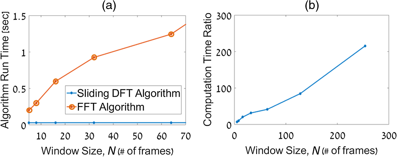

The runtime results for $N=5$, 8, 16, 32, and 64 frames are shown in Fig. 3(a). While the algorithm based on performing an FFT on each window became slower when the number of frames increased, the sliding-DFT algorithm was evidently hardly affected by the number of frames. For $N=5$, the FFT average run time was 201 ms, which was already too slow to produce video-rate calculation time (25 to 30 fps). In contrast, the sliding-DFT algorithm runtime for the same window size was 29 ms, which is sufficient for video-rate processing of PT signals. For $N=64$ frames runtimes were 1240 and 30 ms for FFT and sliding-DFT algorithms, accordingly.

From Fig. 3(b), we can see an increase in the ratio of the FFT and sliding-DFT computation times as the number of frames increases. This trend demonstrates clearly the advantage of implementing sliding DFT in dynamic PTI, especially for a large number of frames. Using the sliding-DFT algorithm with a small window of five frames was 6.9 times faster than the conventional FFT algorithm, which represents a significant improvement. For a window size of 16 frames, already a ratio of 20 was measured, whereas for larger windows even several orders of magnitude of improvement were achieved.

3.2.

Windowing

With large time windows, we get more data, hence enhancing the SNR, but the dynamic nature of the sample may cause smearing of the signal due to sample movement within that time frame. Therefore, we first qualitatively analyzed the signal appearance while changing the number of frames in the window in relation to frame rate and excitation frequency.

In order to test a wide range of window sizes $N$ without smearing the signal too much, we chose a relatively slow moving cell that moved at a speed of $200\mu \mathrm{m}/\mathrm{s}$. The acquisition frame rate of the camera was 2000 fps and the excitation frequency was set at 900 Hz. In Fig. 4, we compare the PTI of the same frame as calculated with two different window sizes. As evident from Figs. 4(a) and 4(c), the signal is stronger and wider when we increase $N$, where a true signal should appear. From Figs. 4(b) and 4(d), however, we see that for a larger window, a false signal appears at the edges of the moving cell, caused by the movement itself, as explained in Sec. 3.

Fig. 4

PT signals at a temporal window size of (a, b) $N=8$ frames, (c, d), $N=64$ frames, and the corresponding quantitative phase images of the same cell as imaged by each mirrors individually. The excited cell is in (a, c, e) and the nonexcited cell with opposite (negative) phase values is in (b, d, f). Dashed red lines indicate the location of the cross-section graphs shown in Fig. 5.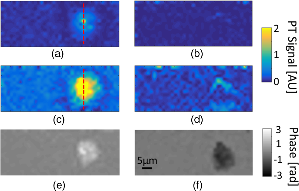

The graphs in Fig. 5 show the cross-section of a PT true signal smear (in pixel units) and the signal rise as a function of window size. As expected, both the SNR [Fig. 5(a)] and smearing [Fig. 5(b)] increased for larger windows. Note that the large FWHM for $N=5$ that can be seen in Fig. 5(c) is caused by the low SNR and the proximity of the signal maximum to the noise floor. The exact optimal window size is specific for a certain system and an experiment setup. It is generally recommended to work with the smallest window size that still produces clear signals. For our measurements, we have found that $N=16$ achieves acceptable results.

Fig. 5

Cross-sections of the PTI images at the middle of the cell, indicated by the dashed red line in Figs. 4(a) and 4(c), as calculated with different values of window size $N$. In (a), the PT signals shown are on the same scale, in (b) the self-normalized signals are shown. In (c), both the FWHM and maximum PT signal as a function of $N$, normalized to the maximal value, are shown.

3.3.

Dynamic PTI with Noise Reduction

As proposed in Sec. 3, the false signals evident in Fig. 4(d) can be significantly reduced. This feature of the algorithm is shown in Fig. 6 (Video 2).

Fig. 6

Demonstration of noise reduction on dynamic PTI data. On the top image, white cells are cells under PT excitation and black cells are with no excitation. (Video 2, MP4, 10.9 MB [URL: http://dx.doi.org/10.1117/1.JBO.22.6.066012.2]).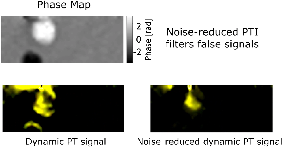

In this video, the brighter cells are the ones that are stimulated by the light of the excitation beam and are expected to form PTI signals, whereas the darker cells, or reference cells, are not influenced by the beam and should not form any distinct spectral signal on the excitation frequency. At first, only the excitation frequency bin is considered, and we do see strong “ghost” signals at the edges of the cells moving in the flow direction. These signals are more visible around the reference cells as they produce no real PT signal, but they do also appear on the excited cells as well. Since these signals are spectrally broadband, an increase of the excitation frequency spectral data is accompanied by a similar increase at the neighboring bins. Therefore, dividing the excitation frequency bin by a nonexcitation bin identified the real PTI signals that are originated by the presence of nanoparticles, rather than by the impact of cell flow. This is shown in the end of Video 2, where the reference cells pose no signal as a response to the excitation frequency.

4.

Summary and Conclusions

Due to the growing interest in AuNPs and the prospects of using them as biomarkers, improved modalities are needed to explore the LPR-based imaging capabilities that are formed by the particles. Full-field OCT and lock-in methods are capable of dynamic PT imaging of AuNPs but with a tradeoff of high cost. In this paper, we have presented a cost-effective system for full-field dynamic PTI of living cells in flow and an improved algorithm, which is based on a sliding window concept for fast data processing. This cost efficient interferometric phase microscopy approach allows the observation of living cells in flow and rapidly produces series of full phase maps of the entire FOV, in addition to the PT molecular-specific signals.

Our system is based on a simple microscope, with an interferometer add-on at the exit port and a PT excitation arm on the sample. The interferometer is used for phase acquisition of the dynamic samples while the excitation arm triggers the PT effect, which is manifested in phase changes retrieved from cells labeled with functionalized AuNPs. The principle of flowing cells through a microchannel in combination with an adapted alignment of the Michelson-interferometer module enabled the self-referencing concept, in which the same cells have been used as both target and control cells, depending on whether they have been under excitation or not in a certain FOV.

We have shown that for rapid dynamic imaging, it is necessary to analyze a smaller number of frames for each PT map as larger frame numbers may create artifacts of the signal such as smearing of a targeted cell, or a ghost signal of a nontargeted cell, resembling motion-blur in imaging. While the former artifact does not ordinarily affect the detection results of targeted cells, the latter might lead to false-positive readings. We succeeded in eliminating these ghost signals by spectral background deduction and thresholding. Other artifacts shown in Fig. 6 are background flashing, caused by medium flow, as well as actual waves of the liquid originated by the PT effect on the cells. This noise may be further reduced by implementing edge detection algorithms to separate cells from background.

Since every PTI system has its own optimal window size, depending on the target velocity, camera frame rate, and excitation frequency, we conclude that the well-known FFT algorithm, with computational complexity of the order of $N·\log N$, can significantly limit the capabilities of the PT system for real-time imaging. Therefore, we implement a combination of algorithms that eliminates window size dependency frame-by-frame. The Goertzel algorithm is used to calculate only the necessary spectral data from the first $N$ frames. Then, for every frame we apply the sliding-DFT algorithm, the computational complexity is independent of $N$ and can only be related to the number of pixels. We have shown that using this algorithm, the computation time is almost independent of the window size and much faster than the FFT. We could demonstrate processing times in the range of 30 ms per frame while keeping a frame rate of over 30 fps.

The proposed system was set for feasibility studies regarding expanding PTI capabilities to dynamic imaging and has demonstrated $0.2\mathrm{mm}/\mathrm{s}$ flowing speed (using 2000 fps). However, recent imaging flow cytometry methods have the ability of acquiring data of thousands of cells per second with physiological velocities of 10 to $40\mathrm{mm}/\mathrm{s}$. As suggested by Eq. (7), the proposed system is potentially capable of acquiring PTI within these limits. Using an optical microscopy system with a magnification of $5\times$, and camera pixel size of $20\mu \mathrm{m}$, for example, while increasing the frame rate to 4000 fps, the imaging system will be able to handle cells flowing at $16\mathrm{mm}/\mathrm{s}$. It should be noted, however, that the trade-off between throughput and resolution should be taken into consideration per application. Further adjustments of the optical parameters of the system, using similar techniques utilized in imaging flow cytometry to increase throughput,²⁵ are expected to allow faster flowing speeds in PTI as well.

This analysis is valid for fast acquisition of PTI for off-line efficient processing. Real-time PTI will still be limited to the processing power of the computer and algorithms, which may be further improved in the future. For instance, we may choose to analyze PT images of only a small ROI, or only choose relevant pixels after image segmentation to further improve the computational analysis time to be smaller than 30 ms per frame, or moreover using graphics processing units for parallel computing.

To conclude, with the emergence of AuNPs as contrast agents and PTI methods for specific molecular imaging, dynamic PTI capabilities are crucial for high-throughput measurements and flow cytometry-based classification of specific cell populations. Toward this goal, we have demonstrated that the proposed method is capable of dynamic, fast-processing PTI, and simultaneously provides rapid processing for regular quantitative imaging, which is essential for deriving cellular parameters, such as volume and dry mass. We thus expect that the proposed dynamic PTI concept will be integrated in future multimodal quantitative phase imaging systems, and will assist in providing specificity in phase imaging of rapidly changing samples, with an option for cell population depletion by PT treatment.