Optical surgical instrument tracking system based on the principle of stereo vision

Zhentian Zhou; Bo Wu; Juan Duan; Xu Zhang; Nan Zhang; Zhiyuan Liang

doi:10.1117/1.JBO.22.6.065005

28 June 2017 Optical surgical instrument tracking system based on the principle of stereo vision

Zhentian Zhou, Bo Wu, Juan Duan, Xu Zhang, Nan Zhang, Zhiyuan Liang

Author Affiliations +

Journal of Biomedical Optics, Vol. 22, Issue 6, 065005 (June 2017). https://doi.org/10.1117/1.JBO.22.6.065005

Abstract

Optical tracking systems are widely adopted in surgical navigation. An optical tracking system is designed based on the principle of stereo vision with high-precision and low cost. This system uses optical infrared LEDs that are installed on the surgical instrument as markers and a near-infrared filter is added in front of the Bumblebee2 stereo camera lens to eliminate the interference of ambient light. The algorithm based on the region growing method is designed and used for the marker’s pixel coordinates’ extraction. In this algorithm, the singular points are eliminated and the gray centroid method is applied to solve the pixel coordinate of the marker’s center. Then, the marker’s matching algorithm is adopted and three-dimensional coordinates’ reconstruction is applied to derive the coordinates of the surgical instrument tip in the world coordinate system. In the simulation, the stability, accuracy, rotation tests, and the tracking angle and area range were carried out for a typical surgical instrument and the miniature surgical instrument. The simulation results show that the proposed optical tracking system has high accuracy and stability. It can meet the requirements of surgical navigation.

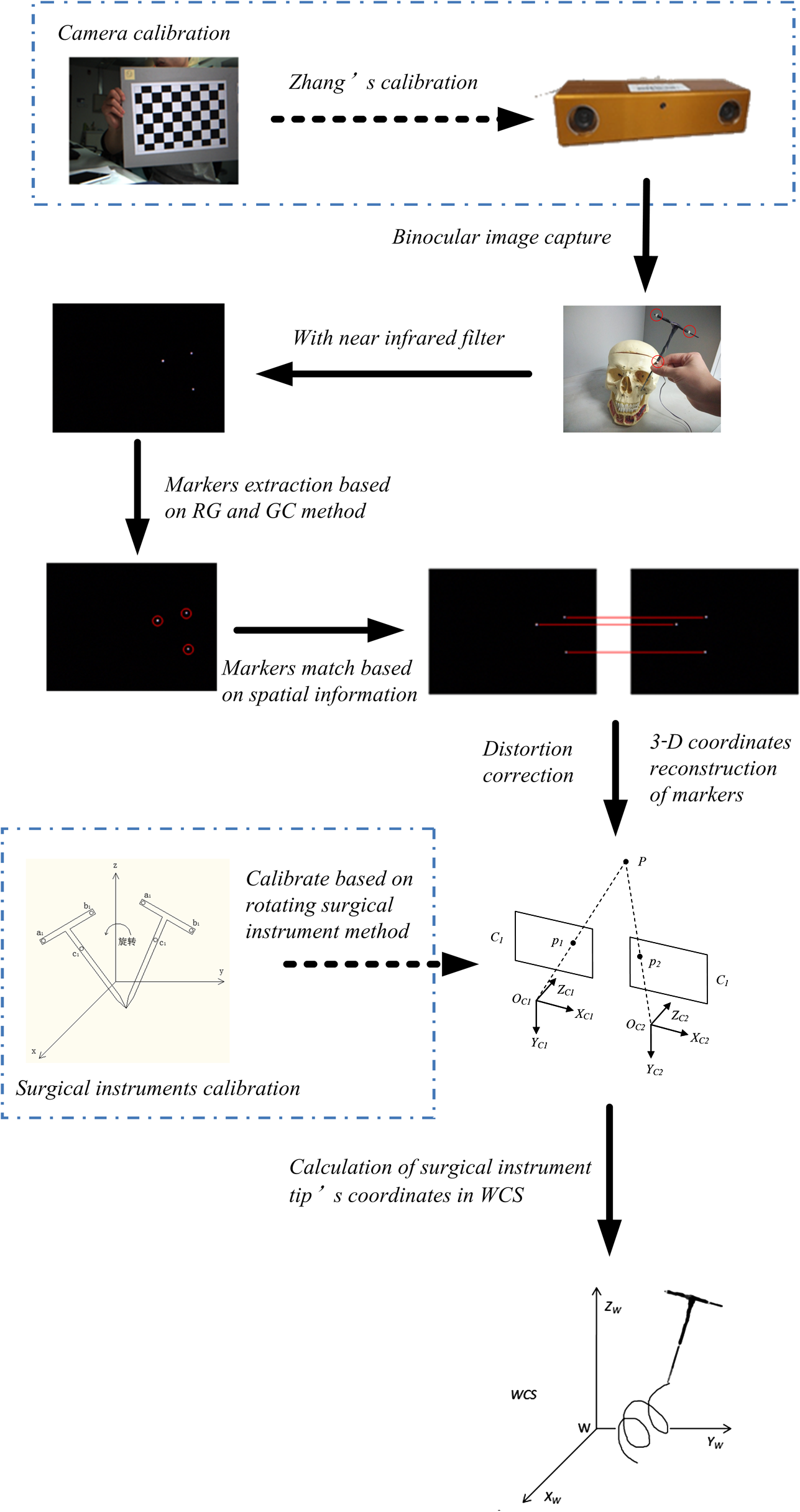
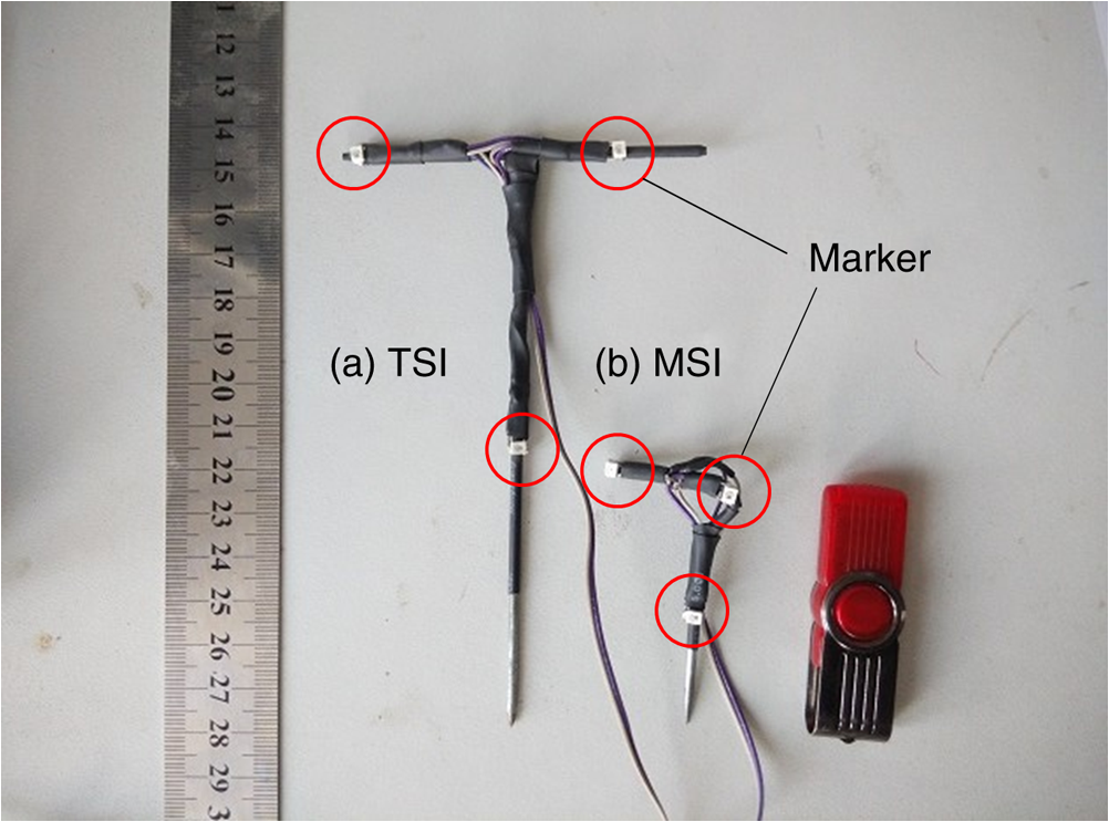
1. Introduction

An image-guided surgical navigation system breaks through the limits of the traditional surgical operation and extends the doctors’ limited vision scope.¹^,² Tracking and positioning are the key techniques of an image-guided surgical navigation system. The accuracy of the tracking method directly determines the accuracy of the image-guided surgical navigation system. An optical tracking system is designed, using light-emitting markers, combined with self-developed image processing methods and an easy-to-implement three-dimensional (3-D) space tracking algorithm, which achieves the high tracking accuracy of surgical instruments.

The tracking methods most widely adopted in image-guided surgical navigation systems include articulated arms, active or passive optical tracking systems, sonic digitizers, and electromagnetic sensors.²^–⁵ Nowadays, the most promising tracking methods are optical and electromagnetic tracking. However, compared with optical tracking, electromagnetic navigation has less precision and its magnetic field is prone to distortion by large metal objects which bring measurement errors to the system.³^,⁶ The commercial optical tracking systems currently used in surgical navigation products mainly include micron tracker (Claron Technology Inc., Canada),⁷ polaris optical tracking systems (Northern Digital Inc., Canada),⁸ StealthStation system (Medtronic Inc., United States),⁹ etc. Unfortunately, these products are always expensive and they are not convenient for further development and customization due to proprietary techniques.

Based upon stereotactic surgery principles, this paper proposes an optical tracking system with low cost and high precision. In the proposed optical tracking system, three optical LEDs are used as the markers that are installed on the surgical instrument. This system uses the Bumblebee2 binocular camera to capture the images of markers. To eliminate the interference of ambient light, a near-infrared filter is added in front of the camera lens. To extract the pixel coordinate of a marker’s center, the region growing (RG) method is used to eliminate the singular point and then the gray centroid (GC) method is adopted to obtain the pixel coordinate of the marker’s center. This image processing method greatly enhances the antijamming capability and improves the accuracy of the system. Next, the algorithm matches the markers in the left and right camera images based on the sequence of its spatial positions. As a last step, it derives the coordinates of the surgical instrument tip by 3-D coordinates reconstruction of markers and realizes the tracking system. Through simulation, the accuracy and stability of system has been verified and can meet the needs of surgical navigation.

2. Methods

2.1.

Framework

The framework of the proposed optical tracking system, which includes the main and auxiliary processes, is shown in Fig. 1. The auxiliary processes consist of the camera calibration and surgical instruments’ calibration that are denoted within the dotted line. This helps the main process obtain the parameters for calculating the coordinates of the markers and the surgical instrument’s tip. For the main process, the stereo camera first captures the binocular images of the surgical instrument. Next, the markers’ extraction, markers’ matching, distortion correction, and 3-D coordinates’ reconstruction procedures are applied to calculate the world coordinates of markers. Finally, the world coordinates of the surgical instrument’s tip can be deduced by the world coordinates of the markers.

Fig. 1

Framework of optical tracking system. The solid line represents the main process and the dotted line represents auxiliary processes that provide several parameters before the main process.

2.2.

Camera Calibration

Zhang’s calibration method¹⁰ is widely used in camera calibration in recent years and is mature. It is a compromise method for traditional camera calibration and self-calibration. This method is robust and it is not necessary to develop a high-precision positioning reference. More importantly, as the calibration accuracy can meet the requirements, Zhang’s method is used to calibrate cameras. The specific calibration tool is the camera calibration toolbox.¹¹ A $5 \times 8$ chessboard is designed as the calibration board; as shown in Fig. 2, the size of each square is $30 \times 30 {mm}^{2}$ .

Fig. 2

Calibration board.

2.3.

Binocular Image Capture

A Bumblebee2 stereo camera¹² is the binocular vision acquisition device adopted in this system. As shown in Fig. 3, two near-infrared filters are installed in front of the camera lens to remove the interference of ambient light.

Fig. 3

Acquisition device of binocular vision.

According to the practical requirements,² two kinds of surgical instruments are designed and employed in the proposed system. They are typical surgical instrument (TSI) and miniature surgical instrument (MSI). TSI is suitable for most cases, while the MSI is suitable for surgeries with limited operation space. In the simulation, these two kinds of surgical instruments are tested separately. For each surgical instrument, three 850-nm near-infrared LEDs are installed and used as the markers, as shown in Fig. 4.

Fig. 4

Two kinds of surgical instruments (a) TSI and (b) MSI.

The luminance of the three markers is captured by the Bumblebee2 camera and the background is completely filtered out by the near-infrared filter. The visual effects of the captured image with and without the near-infrared filter are shown in Fig. 5. From Fig. 5, it can be seen that the ambient light has been effectively filtered out.

Fig. 5

Effect of the near-infrared filter (a) acquisition image without near-infrared filter and (b) acquisition image with near-infrared filter.

2.4.

Markers Extraction

In an optical tracking system, the pixel coordinate of the marker’s center affects the accuracy of the 3-D space coordinates and the coordinate of the surgical instrument tip directly. In the captured images, the markers are the highlighted regions. The pixel coordinate of the marker’s center is the center of the highlighted region and they are used to calculate the world coordinate of surgical instrument tip. So, an effective algorithm is proposed to extract the pixel coordinate of marker’s center from the highlighted region. This algorithm is based on RG and GC methods as shown in Fig. 6.

Fig. 6

Flowchart of markers extraction algorithm based on the RG and GC method.

First, the RG method is used to seek all highlighted connected regions in the image. In this step, a threshold is used to determine the seed and region growth criterion. Its value is set to half of the maximum pixel in the proposed experience. In order to avoid duplication of the seed search, a flag matrix is adopted. Next, the highlighted connected region is compared with the range of the marker’s area (MAR) to determine whether it is noise or the marker. The noise of the CCD sensor is inevitable.¹³ Noise is usually scattered and is shown as small highlighted regions whose areas are much smaller than the marker in the captured image. Through the pre-experiment, the MAR is set as: [11,74] if the area of a highlighted region is less than 11, it is considered to be a noise. Finally, the GC method is applied to calculate the pixel coordinate of the marker’s center. The equation for the GC method is

Eq. (1)

{\begin{matrix} u = \frac{\sum_{i = 1}^{n} u_{i} \cdot f (u_{i}, v_{i})}{\sum_{i = 1}^{n} f (u_{i}, v_{i})} \\ v = \frac{\sum_{i = 1}^{n} v_{i} \cdot f (u_{i}, v_{i})}{\sum_{i = 1}^{n} f (u_{i}, v_{i})} \end{matrix},

where

(u_{i}, v_{i})

is the

i

’th pixel coordinate in the markers’ area, whose gray value is

f (u_{i}, v_{i})

, and

(u, v)

is the derived pixel coordinate of the marker’s center.

The procedures of the markers’ extraction algorithm are as follows:

1. Read the captured marker image.
2. Initialize the flag matrix to 0, whose size is the same as the marker image.
3. Select a pixel $p_{i j}$ from the marker image in raster scan order. If the flag of $p_{i j}$ is 0 and the value of $p_{i j}$ is greater than the threshold, $p_{i j}$ is set as the seed $s_{k}$ . Otherwise, go to step (3) and select the next pixel.
4. Use the RG method to find the highlighted connected region around the seed $s_{k}$ . If the values of pixels are larger than the threshold which is the same as that in step (3), the flags of those pixels are set to 1 and those pixels are defined as the highlighted connected region.
5. After step (4), if the number of pixels in the highlighted connected region is within the MAR, this region is considered to be a marker. The GC method is then adopted to calculate the pixel coordinate of the marker’s center. The pixel coordinate of the marker’s center is denoted as $(u, v)$ . Otherwise, go to step (3) until all of the pixels are selected.

2.5.

Markers Matching

The proposed optical tracking system is based on a binocular camera. According to the model for 3-D coordinates reconstruction of markers (Sec. 2.6), the spatial positions of a pair of matched markers are required. There are three markers in each of the left and right images, respectively. The marker pairs at the same location in the left and right images must be matched before 3-D reconstruction. The spatial positions of markers are used for matching. The positions of the markers on the surgical instrument are fixed, so the positions of the markers on the image are also fixed. The three markers in the left and right images are sorted according to their positions from top to bottom and left to right. Next, the marker pairs can be matched by matching their sorted order number.

2.6.

Three-Dimensional Coordinates Reconstruction of Markers

The mathematical model¹⁴^,¹⁵ of the camera is as follows, which establishes the relationship between the pixel coordinate of the marker’s center and its 3-D spatial world coordinates

Eq. (2)

[\begin{matrix} u \\ v \\ 1 \end{matrix}] = \frac{1}{Z_{C}} \cdot I \cdot E \cdot [\begin{matrix} X_{W} \\ Y_{W} \\ Z_{W} \\ 1 \end{matrix}],

where

(u, v)

is the pixel coordinate of the marker’s center,

Z_{C}

are the

Z

coordinates of markers in the camera coordinate system, and

(X_{W}, Y_{W}, Z_{W})

are the coordinates of markers in the world coordinate system (WCS), respectively.

I

and

E

are the internal and the external parameters of the camera that can be obtained by camera calibration.

Two equations of Eq. (2) can be established for the binocular stereo camera, as shown in Eq. (3). The world coordinates of markers can be derived from

Eq. (3)

{\begin{matrix} [\begin{matrix} u_{left} \\ v_{left} \\ 1 \end{matrix}] = \frac{1}{Z_{C left}} \cdot I_{left} \cdot E_{left} \cdot [\begin{matrix} X_{W} \\ Y_{W} \\ Z_{W} \\ 1 \end{matrix}] \\ [\begin{matrix} u_{right} \\ v_{right} \\ 1 \end{matrix}] = \frac{1}{Z_{C right}} \cdot I_{right} \cdot E_{right} \cdot [\begin{matrix} X_{W} \\ Y_{W} \\ Z_{W} \\ 1 \end{matrix}] \end{matrix} .

2.7.

Distortion Correction

The pinhole imaging mathematical model used in this paper is an ideal linear mathematical model. In the process of manufacturing and installation, camera lens distortion is inevitable.¹⁶ In order to eliminate the influence of lens distortion on the positioning accuracy, the lens distortion must be corrected. According to the camera model based on Heikkilä and Silvén,¹⁷ the distortion model adopted in this paper is as

Eq. (4)

{\begin{matrix} u^{'} = u + u (k_{1} r^{2} + k_{2} r^{4} + k_{3} r^{6}) + p_{1} (3 u^{2} + v^{2}) + 2 p_{2} u v \\ v^{'} = v + v (k_{1} r^{2} + k_{2} r^{4} + k_{3} r^{6}) + 2 p_{1} u v + p_{2} (u^{2} + 3 v^{2}) \end{matrix},

where

(u^{'}, v^{'})

,

(u, v)

are the actual and the ideal pixel coordinates of a marker’s center,

r^{2} = u^{2} + v^{2}

.

k_{1}

,

k_{2}

, and

k_{3}

are the radial distortion coefficients, and

p_{1}

,

p_{2}

are the centrifugal distortion coefficients.

To verify the effect of the camera lens distortion correction module in the proposed optical tracking system, an experiment is carried out. Three kinds of distances, which are short, medium, and long, are measured by the proposed tracing system. For each kind of distance, the endpoints’ coordinates are measured using the distortion correction model and the nondistortion correction model. Each distance is measured 50 times and the average value is calculated. The actual distance is measured by using a Vernier caliper. The distances measured by the tracking system are compared with the actual distances. The error is the difference between them as shown in Table 1.

Table 1

Comparison of the results of distortion correction and nondistortion correction.

Number	Distortion correction (mm)	Nondistortion correction (mm)	Actual distance (mm)	Error (mm)
Number	Distortion correction (mm)	Nondistortion correction (mm)	Actual distance (mm)	Distortion correction	Nondistortion correction
1	9.48	9.45	9.50	0.02	0.05
2	22.01	22.16	22.02	0.01	0.14
3	37.68	37.90	37.70	0.02	0.20

From Table 1, it can be seen that the distortion correction errors are smaller than the nondistortion correction error. With the increasing of distance, the distortion correction error becomes smaller.

2.8.

Surgical Instrument Calibration

The purpose of optical tracking is to obtain the world coordinates of the surgical instrument’s tip. Through 3-D reconstruction, the world coordinates of the markers can be obtained. According to the shape of a surgical instrument, a surgical instrument coordinate system (SICS) can be established, as shown in Fig. 7.

Fig. 7

SICS.

The coordinates of the surgical instrument tip in SICS are $P_{tip_s}$ $(X_{tip_s}, Y_{tip_s}, Z_{tip_s})$ , and $P_{tip_w}$ $(X_{tip_w}, Y_{tip_w}, Z_{tip_w})$ in WCS. The rotation matrix and the translation matrix of SICS with respect to WCS are $R$ and $T$ , then

Eq. (5)

P_{tip_w} = R P_{tip_s} + T .

R

and

T

can be calculated by markers’ coordinates

m_{1}

,

m_{2}

, and

m_{3}

(Ref. 18)

Eq. (6)

T = m_{1} + \frac{\vec{m_{1} m_{3}} \cdot \vec{m_{1} m_{2}}}{{‖ m_{1} m_{2} ‖}^{2}} \cdot \vec{m_{1} m_{2}},

Eq. (7)

R = [\begin{matrix} \frac{\vec{o m_{3}}}{‖ \vec{o m_{3}} ‖} & \frac{\vec{o m_{2}}}{‖ \vec{o m_{2}} ‖} & \frac{\vec{o m_{3}}}{‖ \vec{o m_{3}} ‖} \times \frac{\vec{o m_{2}}}{‖ \vec{o m_{2}} ‖} \end{matrix}],

where the coordinates of

o

are numerically equal to

T

.

The purpose of the surgical instrument calibration is to get the coordinates of $P_{tip_s}$ . Equations (5)–(7) are used to calculate the world coordinates of the surgical instrument tip by markers’ world coordinates.

The rotating surgical instrument method¹⁶ is used to get $P_{tip_s}$ . The idea is to fix the position of the surgical instrument tip and rotate the surgical instrument. Thus, the same marker on the surgical instrument satisfies the spherical equation [Eq. (8)], in which the coordinates of a surgical instrument tip are the center of the sphere. The world coordinates of the surgical instrument tip can be obtained by solving Eq. (10). Assuming $n$ images are obtained by rotating the surgical instrument, the coordinate of the $i$ ’th marker and in the $j$ ’th image in the WCS is defined as $P_{i j} (X_{i j}, Y_{i j}, Z_{i j})$ $(i = 1, 2, 3; j = 1, 2, \dots, n)$ . The world coordinates of the tip are denoted as $(X_{tip_w}, Y_{tip_w}, Z_{tip_w})$ . Under the rigid body constraint, the distance between $P_{tip_w}$ and $P_{i j}$ is $ρ$

Eq. (8)

{(X_{i j} - X_{tip_w})}^{2} + {(Y_{i j} - Y_{tip_w})}^{2} + {(Z_{i j} - Z_{tip_w})}^{2} = ρ_{i}^{2} .

Eq. (8) has

i \times j

equations. For each

i

, using the

j

’th (

j \geq 2

) equation minus the (

j - 1

)’th equation, the following equation can be obtained

Eq. (9)

[X_{i j} - X_{i (j - 1)}] X_{tip_w} + [Y_{i j} - Y_{i (j - 1)}] Y_{tip_w} + [Z_{i j} - Z_{i (j - 1)}] Z_{tip_w} = \frac{1}{2} [X_{i j}^{2} - X_{i (j - 1)}^{2} + Y_{i j}^{2} - Y_{i (j - 1)}^{2} + Z_{i j}^{2} - Z_{i (j - 1)}^{2}] .

Eq. (9) has

i \times (j - 1)

equations, which can be expressed in a matrix form

Eq. (10)

W P_{tip_w} = F .

Among them,

W

is an

i \times (j - 1)

row by three columns of the matrix and

F

is the

i \times (j - 1)

vectors. When

j \geq 2

, Eq. (10) is an over determined equation, and the least square method can be used to solve

P_{tip}

.

In this paper, the calibration is carried out by 20 rotating surgical instruments. The $i$ ’th rotation matrix and the translation matrix of the SISC relative to the WCS are $R_{i}$ and $T_{i}$ , and the tip coordinate can be calculate by

Eq. (11)

P_{tip_s} = R_{i}^{- 1} (P_{tip_w} - T_{i}) .

3. Simulation Results

In order to verify and determine the stability and accuracy of the system, the stability, space distance, and rotation tests were carried out for TSI and MSI. The stability experiment is designed to measure the system stability under the condition of repeated measurement. The accuracy of the system is measured by a space distance experiment. The absolute error is compared by the results of calculated distance between two points and a Vernier caliper. Furthermore, the stability and accuracy of the tip coordinates are tested by a rotation experiment at different angles.

3.1.

Calibration Settings

Twenty pairs of the left and right images of the calibration board are captured at different locations as shown in Fig. 8. Internal and external parameters of camera calibration of each camera are $I_{left}$ , $I_{right}$ and $E_{left}$ , $E_{right}$ , respectively

I_{left} = [\begin{matrix} 815.8132 & 0 & 310.9348 \\ 0 & 819.2989 & 246.9482 \\ 0 & 0 & 1 \end{matrix}],

I_{right} = [\begin{matrix} 815.0779 & 0 & 314.2526 \\ 0 & 818.7035 & 243.6091 \\ 0 & 0 & 1 \end{matrix}],

E_{right} = [\begin{matrix} 1 & - 0.0003 & - 0.0039 & - 119.6752 \\ 0.0003 & 1 & 0.0027 & 0.0236 \\ 0.0039 & - 0.0027 & 1 & - 0.0209 \end{matrix}] .

Fig. 8

Camera calibration images (a) left camera calibration images and (b) right camera calibration images.

The left camera’s optical center is used as the origin of the WCS. In this system, $E_{left}$ is a fixed value, as shown

E_{left} = [\begin{matrix} 1 & 0 & 0 & 0 \\ 0 & 1 & 0 & 0 \\ 0 & 0 & 1 & 0 \end{matrix}] .

3.2.

Stability Test

When the optical tracking system is working, the system must have sufficient stability. If the surgical instrument remains still, the calculated tip coordinates may change due to the changes in the capture environment and the stability of the algorithm. In order to test the stability of the system, 10 different position points are selected randomly and the surgical instrument is kept still in each position. For each position, 100 sets of images are used for repeating. Then, the standard deviations (SD) of $X$ -, $Y$ -, and $Z$ -directions are calculated, respectively, which are used to evaluate the stability of the system. Two kinds of surgical instruments are tested in the experiment. The results are shown in Table 2. Figure 9 shows another representation of Table 2 for MSI.

Table 2

The coordinates stability results for TSI and MSI.

	TSI				MSI
Position no.	X-direction SD (mm)	Y-direction SD (mm)	Z-direction SD (mm)	Position no.	X-direction SD (mm)	Y-direction SD (mm)	Z-direction SD (mm)
1	0.01180	0.00731	0.09218	1	0.01442	0.00834	0.07428
2	0.01402	0.00618	0.07680	2	0.01064	0.00846	0.06335
3	0.01821	0.00823	0.07869	3	0.01104	0.00892	0.06879
4	0.01449	0.00954	0.08518	4	0.01072	0.00787	0.05100
5	0.01278	0.00579	0.07710	5	0.01436	0.01148	0.08619
6	0.01610	0.00794	0.09708	6	0.01116	0.01099	0.07057
7	0.01748	0.00757	0.05763	7	0.01003	0.00839	0.05106
8	0.02377	0.00844	0.08088	8	0.01424	0.00915	0.05962
9	0.01635	0.00764	0.07070	9	0.01556	0.01027	0.05574
10	0.03487	0.00967	0.09490	10	0.01677	0.01037	0.09452
Average	0.01799	0.00783	0.08112		0.01289	0.00942	0.06751

Fig. 9

The 3-D coordinate stability results for MSI. (a) Results of the $X$ -direction measurement, the range of $X$ -direction SD is from 0.01003 to 0.01677, and the range of $X$ -direction CV is from 0.012% to 0.068%; (b) results of the $Y$ -direction measurement, the range of $Y$ -direction SD is from 0.00787 to 0.01148, and the range of $Y$ -direction CV is from 0.011% to 0.016%; and (c) results of the $Z$ -direction measurement, the range of $Z$ -direction SD is from 0.05100 to 0.09452, and the range of $Z$ -direction CV is from 0.014% to 0.027%.

From the above results, it can be seen that the average SDs of the $X$ -, $Y$ -, and $Z$ -directions in 10 positions are 0.01799, 0.00783, 0.08112 mm for TSI and 0.01289, 0.00942, 0.06751 mm for MSI, respectively. In Table 2, the worst results are 0.09708 and 0.09452 mm for two different instruments.

From Fig. 8, it also can be seen that the range of the $X$ coordinate is about (45, 75 mm), the range of the $Y$ coordinate is about (150, 153 mm), and the range of the $Z$ coordinate is about (330, 390 mm). As a result, it looks like that the SD of the $Z$ -direction is bigger than the other two directions, but the coefficient of variations (CVs) of the three directions from Fig. 9 are almost the same range.

3.3.

Space Distance Test

Since the absolute coordinates obtained by the optical tracking system are in the WCS, it is difficult to directly evaluate the accuracy of the world coordinates. Therefore, in order to test the position accuracy of the simulated surgical instruments, this system adopts the method of indirect measurement. Within the scope of the effective field of the optical tracking system, the tip coordinates in the two places are randomly chosen and the distances are measured. Then, the tracking accuracy of the system is evaluated by comparing the distance with the actual measured distance using a Vernier caliper and grating ruler.

Ten groups of different distances were measured, respectively, by Vernier caliper and grating ruler that includes short distance, medium distance, and long distance, and each tip coordinate is measured 50 times. The average absolute errors using the Vernier caliper are shown in Figs. 10 and 11. The average absolute errors of two surgical instruments measured by Vernier caliper are 0.23 and 0.13 mm.

Fig. 10

Space distance test result of TSI by vernier caliper. (a) Results of the short-distance (0 to 15 mm) measurement, compare the calculated and measured distance, the range of space distance error is from 0.18 to 0.38 mm; (b) results of the medium-distance (20 to 40 mm) measurement, compare the calculated and measured distance, the range of space distance error is from 0.19 to 0.34 mm; and (c) results of the long-distance (40 to 55 mm) measurement, compare the calculated and measured distance, the range of space distance error is from 0.13 to 0.26 mm.

Fig. 11

Space distance test result of MSI by vernier caliper. (a) Results of the short-distance (0 to 10 mm) measurement, compare the calculated and measured distance, the range of space distance error is from 0.06 to 0.10 mm; (b) results of the medium-distance (10 to 20 mm) measurement, compare the calculated and measured distance, the range of space distance error is from 0.06 to 0.19 mm; and (c) results of the long-distance (20 to 25 mm) measurement, compare the calculated and measured distance, the range of space distance error is from 0.13 to 0.20 mm.

However, the accuracy results of the proposed optical tracking system have more than four decimal places. To compare with the results of the Vernier caliper, the last several decimal places have been rounded. In order to evaluate the accuracy of the proposed optical tracking system more accurately, we use a more accurate measurement device, a grating ruler. The brand of grating ruler is SION, and the model is KA-300/5U/1020 mm.

The “grating ruler” is rigidly fixed on the “precision optical table” to ensure the stability, and then the TSI or MSI is also fixed to the grating ruler, as shown in Figs. 12 and 13. The results measured by Vernier caliper are used as a reference, and the new distance measurement values are determined by using the grating ruler, as shown in Tables 3 and 4, and Fig. 14. From Tables 3 and 4, it can be seen that higher measurement accuracy is obtained by using the grating ruler. The fluctuation range of the distance root mean square error (RMSE) becomes smaller as shown in Fig. 14.

Fig. 12

Diagram of precision optical table and the TSI fixed on the grating ruler.

Fig. 13

Diagram of the MSI fixed on the grating ruler.

Table 3

Space distance test results for TSI.

	Group 1 vernier caliper				Group 2 grating ruler
Position no.	Measured by vernier caliper (mm)	Calculated by the proposed system (mm)	Absolute distance error (mm)	Distance RMSE	Measured by grating ruler (mm)	Calculated by the proposed system (mm)	Absolute distance error (mm)	Distance RMSE
1	6.64	6.43	0.21	0.33	6.64	6.699	0.059	0.063
2	7.66	7.28	0.38	0.40	7.665	7.698	0.033	0.040
3	14.68	14.50	0.18	0.26	14.685	14.665	0.020	0.031
4	24.62	24.40	0.22	0.29	24.625	24.629	0.004	0.020
5	33.04	32.85	0.19	0.26	33.045	33.076	0.031	0.036
6	35.10	35.32	0.22	0.32	35.1	35.041	0.059	0.062
7	39.36	39.02	0.34	0.37	39.36	39.336	0.024	0.035
8	41.86	41.99	0.13	0.32	41.865	41.877	0.012	0.026
9	42.42	42.68	0.26	0.35	42.425	42.369	0.056	0.059
10	53.34	53.54	0.20	0.34	53.345	53.457	0.112	0.117
Average			0.23	0.32			0.041	0.049

Table 4

Space distance test results for MSI.

Position no.	Group 1 vernier caliper				Group 2 grating ruler
Position no.	Measured by vernier caliper (mm)	Calculated by the proposed system (mm)	Absolute distance error (mm)	Distance RMSE	Measured by grating ruler (mm)	Calculated by the proposed system (mm)	Absolute distance error (mm)	Distance RMSE
1	5.82	5.76	0.06	0.02	5.775	5.803	0.028	0.035
2	9.12	9.22	0.10	0.02	9.245	9.282	0.037	0.041
3	13.46	13.61	0.15	0.02	13.625	13.615	0.010	0.020
4	15.08	14.91	0.17	0.10	14.915	14.894	0.021	0.026
5	15.02	15.08	0.06	0.12	15.105	15.096	0.009	0.023
6	15.46	15.27	0.19	0.12	15.315	15.276	0.039	0.043
7	15.90	15.82	0.08	0.10	15.845	15.855	0.010	0.016
8	21.12	21.26	0.14	0.12	21.275	21.272	0.003	0.018
9	22.06	21.86	0.20	0.12	21.895	21.857	0.038	0.046
10	22.08	22.21	0.13	0.13	22.265	22.220	0.045	0.050
Average			0.13	0.09			0.024	0.032

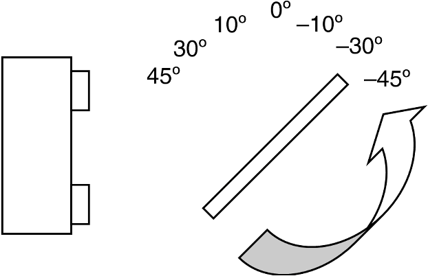
Fig. 14

Fluctuation ranges of distance RMSE for TSI and MSI. (a) Fluctuation ranges of distance RMSE for TSI and (b) fluctuation ranges of distance RMSE for MSI.

The average absolute distance error is 0.23 mm for TSI and 0.13 mm for MSI by Vernier caliper, 0.041 mm for TSI and 0.024 mm for MSI by grating ruler, respectively. The distance RMSE is 0.32 mm for TSI and 0.09 mm for MSI by Vernier caliper, 0.049 mm for TSI and 0.032 mm for MSI by grating ruler, respectively. The results show that the proposed optical tracking system has a higher accuracy and it can meet the accuracy requirement of space tracking equipment in surgical navigation.

3.4.

Rotation Test

In the rotational experiment, the stability of the rotation of the surgical instrument and the angular accuracy of the rotation angle are tested.

When the camera captures the marker images from different angles, the size of the marker in the image is constantly changing. In order to verify that the calculated coordinates are accurate for any capturing angle, a rotating stability experiment is designed. Because the size of the MSI is too small to do the experiment, only the TSI is done for this test. As shown in Fig. 15, the tip of the TSI is fixed. Then, let the TSI rotate from $- 45 \deg$ to 45 deg. Every angle is measured 100 times and the values of the tip coordinates are averaged. In this experiment, the tip of the TSI did not move, so its coordinates in different angles are constant in theory. Seven different rotation angles are tested, and the tip coordinates are shown in Table 5.

Fig. 15

Angle schematic diagram of rotational stability.

Table 5

Coordinates for the TSI tip in different rotation angles.

Angle (deg)	X coordinates (mm)	Y coordinates (mm)	Z coordinates (mm)
$- 45$	84.22881	195.97334	366.77527
$- 30$	84.08752	196.58719	366.35975
$- 10$	84.04392	196.56368	366.32654
0	84.10147	196.08926	367.30858
10	84.00152	196.54439	366.84694
30	84.05953	196.46245	366.81637
45	84.18887	195.99652	366.85869

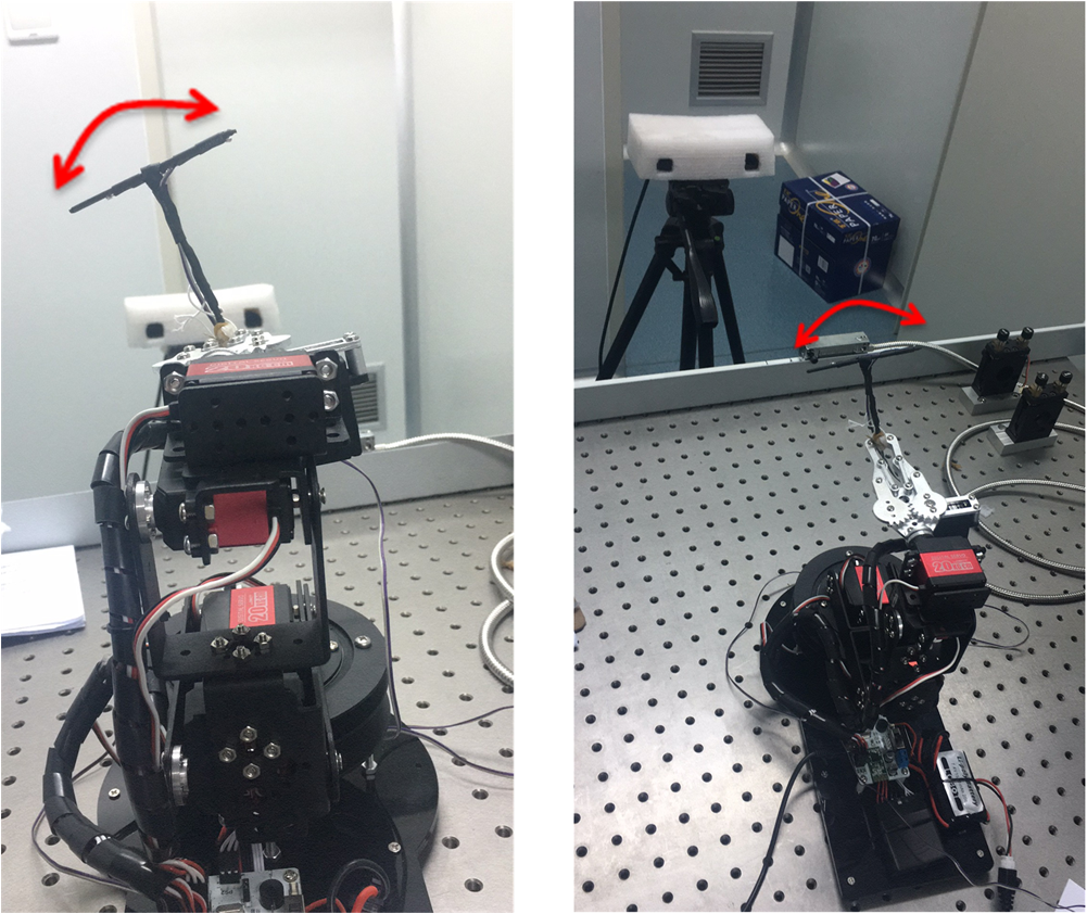
The SDs of the coordinates of the TSI tip in different rotation angles are 0.08074, 0.28266, and 0.33407 mm in the $X$ -, $Y$ -, and $Z$ -directions, respectively. From the above data, it can be seen that the coordinates of the tip do not change significantly, which shows that the proposed tracking algorithm is accurate enough to guarantee the coordinates of the TSI tip to be unchanged under different capturing angle conditions. The proposed tracking system has a high rotational stability.

In order to get a more accurate rotation angle, TSI or MSI is fixed on the 6-DOF mechanical arm. The brand of the 6-DOF mechanical arm is LOBOT, and the model is MK12352. Twelve angle groups are measured from 5 deg to 60 deg. Every angle is measured 100 times by TSI or MSI, and then averaged. The rotation angle is measured as indicated by the red arrow in Fig. 16 and the results are shown in Table 6. From Table 6, it can be seen that the absolute error of the average angle of 12 groups is 0.36 deg for TSI and 0.28 deg for MSI, respectively.

Fig. 16

Diagram of TSI fixed on a 6-DOF mechanical arm.

Table 6

Rotation angle measurement result.

Rotation no.	Group 1 TSI					Group 2 MSI
Rotation no.	Measured by 6-DOF mechanical arm (deg)	Calculated by TSI (deg)	Rotation angle absolute error (deg)	Rotation angle RMSE	Rotation no.	Measured by 6-DOF mechanical arm (deg)	Calculated by MSI (deg)	Rotation angle absolute error (deg)	Rotation angle RMSE
1	5.04	4.75	0.29	0.31	1	5.04	4.79	0.25	0.31
2	10.08	9.45	0.63	0.64	2	10.08	10.37	0.29	0.34
3	15.12	15.04	0.08	0.16	3	15.12	14.80	0.32	0.41
4	20.16	20.14	0.02	0.12	4	20.16	20.30	0.14	0.24
5	25.20	24.35	0.85	0.85	5	25.20	24.87	0.33	0.41
6	30.24	29.45	0.79	0.79	6	30.24	30.57	0.33	0.40
7	35.28	35.40	0.12	0.16	7	35.28	35.61	0.33	0.37
8	40.32	40.04	0.28	0.32	8	40.32	40.03	0.29	0.34
9	45.36	44.87	0.49	0.50	9	45.36	45.57	0.21	0.26
10	50.40	49.85	0.55	0.56	10	50.40	50.01	0.39	0.41
11	55.44	55.30	0.14	0.19	11	55.44	55.13	0.31	0.38
12	60.48	60.57	0.09	0.21	12	60.48	60.29	0.19	0.28
Average			0.36	0.40	Average			0.28	0.35

3.5.

Tracking Angle and Area Range Test

The tracking angle view and area range of the proposed optical tracking system are shown in Figs. 17 and 18, respectively.

Fig. 17

The angle view range of the proposed optical tracking system. (a) The angle view range for TSI. (b) The angle view range for MSI.

Fig. 18

The spatial measurement range of the proposed optical tracking system. (a) The spatial measurement range for TSI. (b) The spatial measurement range for MSI.

The angle view range is limited by the instrument on which there are only three markers. Rotation around the $Z$ -axis ranges from $- 78.3383 \deg$ to 74.6440 deg for TSI, and from $- 67.9872 \deg$ to 53.9503 deg for MSI, which is the red area in Fig. 17. Rotation around the $X$ -axis ranges from $- 86.2429 \deg$ to 88.1640 deg for TSI, and from $- 87.9051 \deg$ to 89.0361 deg for MSI, which is the green area in Fig. 17. Rotation around the $Y$ -axis ranges from $- 74.2184 \deg$ to 75.04111 deg for TSI, and from $- 57.4553 \deg$ to 73.4661 deg for MSI, which is the blue area in Fig. 17.

The measurement of height and width depends on the distance in the $Z$ -direction. In the $Z$ -direction (from near to far), the common distance ranges from 219.0297 to 2577.6776 mm for TSI, from 198.5920 to 612.5765 mm for MSI, respectively. The occasionally farthest distance that can be measured is 3022.9473 mm for TSI and 2954.3603 mm for MSI, which is shown as the blue point in Fig. 18. The dashed line space is more precise than the solid line space, which can be measured with more instrument poses.

Through the system experiment, the measurable range of the proposed optical tracking system is sufficient to meet the scope of surgical navigation.

3.6.

Cost Estimation

Polaris Spectra and Polaris Vicra system are popular commercial surgical tracking system, from Northern Digital Inc. (NDI) company. The prices are different for different types of the system, e.g., systems with active or passive markers. The cheapest is more than $31,340, the most expensive one is $52,496.

The optical positioning system proposed in this paper mainly includes a 1394 card, binocular camera, LED marker, infrared filter, wires, proposed positioning software system, and so on. The cost estimation of the proposed optical tracking system is $3,366 as shown in Table 7.

Table 7

Cost estimation of proposed optical tracking system.

Device name	Cost estimation	Amount	Total cost estimation
Bumblebee2 (binocular camera)	$3237	1	$3237
LED maker	$0.03	3	$0.1
Infrared filter	$5	2	$10
1394 card	$4	1	$4
Proposed positioning software system	$100	1	$100
Wires	$15	*	$15
Estimated total price			$3366.1

The note * in Table means it is an estimation of the wires used in our system. It depends in practical applications.

Taking into account the ratio between cost and commercialization, if the ratio is 3, the total price is $10,000. It substantially reduces the price compared with the existing commercial tracking systems.

4. Discussion

In this paper, an optical tracking system based on a Bumblebee2 binocular camera is designed. An 850-nm near-infrared optical LED is used as the marker of surgical instruments. Meanwhile, an infrared filter is installed in front of the camera lens, which can effectively eliminate the interference of ambient light. In the space location algorithm, the RG method is designed to find the highlighted connected region of markers in the image. In order to eliminate the singular point, the pixel coordinate of the marker’s center is calculated by the GC method. With an optical tracking system, it is difficult to match the markers in a traditional way. A matching method for the 3-D reconstruction based on the position order of the markers is proposed, and the results are satisfying. In the end, the rotating surgical instrument method is used to calibrate the surgical instrument to obtain the position relationship between the tip and the SCS, resulting in tracking of the surgical instrument tip.

In the stability experiment, 10 different positions are measured and calculated for the SDs of tip coordinates for TSI and MSI in the $X$ -, $Y$ -, and $Z$ -directions. The worst results of the two kinds of surgical instruments are 0.09708 and 0.09452 mm, respectively. The average value of SDs are 0.01799, 0.00783, 0.08112 mm in the $X$ -, $Y$ -, $Z$ -directions for TSI, and 0.01289, 0.00942, 0.06751 mm for MSI. For the $X$ - and $Y$ -directions, it can be seen that the SD is very small. The SD is slightly larger in the $Z$ -direction because the coordinate is also much larger than in the other two directions. From the CV results of the three directions, the same conclusion can be made. In the space distance experiment, the distance RMSE is 0.32 mm for TSI and 0.09 mm for MSI by Vernier caliper, 0.049 mm for TSI and 0.032 mm for MSI by grating ruler, respectively. The accuracy of Polaris Spectra and Polaris Vicra system of NDI company can achieve 0.25 mm RMS in pyramid.⁸ In the proposed optical tracking system, the measurable distance range is from 219.0297 to 2577.6776 mm for TSI, from 198.5920 to 612.5765 mm for MSI in $Z$ -direction (from near to far). The occasionally farthest distance that can be measured is 3022.9473 mm for TSI and 2954.3603 mm for MSI, respectively. In the existing systems, the measurable distance ranges from 950 to 3000 mm for Polaris Spectra system, from 557 to 1336 mm for Polaris Vicra system in $Z$ -direction. Because the surgical instruments are welded by us and are subject to a limitation because the luminescent marker is oriented in a single direction, the measurable area range of TSI and MSI is not as large as that of the Polaris Spectra system and Polaris Vicra system. However, the nearest measurable locations for TSI and MSI are better than Polaris Spectra and Polaris Vicra systems. It is advantageous for surgical operations that commonly have a small operating view. Through the system experiment, it can be seen that the proposed optical tracking system and the corresponding space tracking algorithm have high stability and accuracy. Moreover, comparing with the cost of the proposed optical tracking system and the existing systems, the price has been greatly reduced.

5. Conclusions

In this paper, a low cost, open optical tracking system based on binocular vision theory is proposed. The system uses the stereo camera and combines with the self-developed image processing methods and easy-to-implement 3-D space tracking algorithm, which accomplishes the high accuracy of surgical instruments tracking. Experimental results show that the system has high stability and accuracy, and it can provide accurate guidance for surgical navigation.

The system and the related algorithm are a meaningful exploration in the field of surgical navigation. Considering the practical application, it has room for improvement. For example, a battery can be used to supply power for the marker, so as to avoid the wire connected to the surgical instruments. The surgical instruments without wire can move more freely. In the future, we will design the power supply circuit for the surgical instruments to install the button batteries. The fast calibration algorithm needs further study. The algorithm of pixel coordinates extraction and the marker matching can also be optimized at the same time, so that the tracking accuracy of the system can be improved. The real-time synchronization needs to be further optimized to achieve higher system accuracy. At present, with more and more accurate operation requirements, the accuracy and stability of the optical tracking system needs continuous improvement.

Disclosures

No conflicts of interest, financial or otherwise are declared by the authors.

Acknowledgments

The authors would like to thank Mr. Hans Hermans for manuscript editing, Boqi Jia and Mengshi Zhang for the new revised experiment, Dr. Yu Wang for helping to buy the equipment of grating ruler and 6-DOF mechanical arm, and we are thankful for Zhang’s calibration method. This work was supported in part by the National Natural Science Foundation of China (No. 61672362 and 61272255), the Beijing Natural Science Foundation (No. 4172012), and the Scientific Research Common Program of Beijing Municipal Commission of Education (No. KM201710025011).

References

1.

A. Wagner et al., “Image-guided surgery,” Int. J. Oral Maxillofac. Surg., 25 (7), 147 –151 (1996). http://dx.doi.org/10.1016/S0901-5027(96)80062-2 IJOSE9 0901-5027 Google Scholar

2.

F. A. Jolesz, Intraoperative Imaging and Image-Guided Therapy, Springer, New York (2014). Google Scholar

3.

M. Maybody, C. Stevenson and S. B. Solomon, “Overview of navigation systems in image-guided interventions,” Tech. Vasc. Interventional Radiol., 16 (3), 136 –143 (2013). http://dx.doi.org/10.1053/j.tvir.2013.02.008 Google Scholar

4.

L. Appelbaum et al., “Image-guided fusion and navigation: applications in tumor ablation,” Tech. Vasc. Interventional Radiol., 16 (4), 287 –295 (2013). http://dx.doi.org/10.1053/j.tvir.2013.08.011 Google Scholar

5.

S. J. Phee and K. Yang, “Interventional navigation systems for treatment of unresectable liver tumor,” Med. Biol. Eng. Comput., 48 (2), 103 –111 (2010). http://dx.doi.org/10.1007/s11517-009-0568-3 Google Scholar

6.

F. Kral et al., “Comparison of optical and electromagnetic tracking for navigated lateral skull base surgery,” Int. J. Med. Rob. Comput. Assist. Surg., 9 (2), 247 –252 (2013). http://dx.doi.org/10.1002/rcs.v9.2 Google Scholar

7.

Claron Technology Inc., “Microntracker[EB/OL],” (2015) http://www.claronav.com/microntracker/ September ). 2015). Google Scholar

8.

Northern Digital Inc., “Polaris optical tracking systems[EB/OL],” (2015) http://www.ndigital.com/medical/products/polaris-family/ September ). 2015). Google Scholar

9.

Medtronic Inc., “Stealth station S7 surgical navigation system[EB/OL],” (2015) http://www.medtronic.com/for-healthcare-professionals/products-therapies/spinal/surgical-navigation-imaging/surgical-navigation-systems/systems-software-instruments/index.htm September ). 2015). Google Scholar

10.

Z. Zhang, “A flexible new technique for camera calibration,” IEEE Trans. Pattern Anal. Mach. Intell., 22 (11), 1330 –1334 (2000). http://dx.doi.org/10.1109/34.888718 Google Scholar

11.

“Camera calibration toolbox for Matlab[EB/OL],” (2015) http://www.vision.caltech.edu/bouguetj/calib_doc/ September ). 2015). Google Scholar

12.

Point Gray Research Inc., “Bumblebee2 1394a[EB/OL],” (2015) http://www.ptgreychina.com//bumblebee2-firewire-stereo-vision-camera-systems September ). 2015). Google Scholar

13.

Y. Reibel et al., “CCD or CMOS camera noise characterization,” Eur. Phys. J. Appl. Phys., 21 (01), 75 –80 (2003). http://dx.doi.org/10.1051/epjap:2002103 Google Scholar

14.

J. W. Yi and J. H. Oh, “Estimation of depth and 3D motion parameter of moving object with multiple stereo images,” Image Vision Comput., 14 (7), 501 –516 (1996). http://dx.doi.org/10.1016/0262-8856(95)01073-4 IVCODK 0262-8856 Google Scholar

15.

U. Dhond and J. Aggarwal, “Structure from stereo-a review,” IEEE Trans. Syst., Man, Cybern., 19 1489 –1510 (1989). http://dx.doi.org/10.1109/21.44067 Google Scholar

16.

C. C. Slama, C. Theurer and S. W. Henriksen, Manual of Photogrammetry, American Society of Photogrammetry, Virginia (1980). Google Scholar

17.

J. Heikkila and O. Silvén, “A four-step camera calibration procedure with implicit image correction,” in Proc. IEEE Computer Society Conf. on Computer Vision and Pattern Recognition, 1106 –1112 (1997). http://dx.doi.org/10.1109/CVPR.1997.609468 Google Scholar

18.

B. Sun et al., “Surgical instrument recognition and calibration for optical tracking system,” in IEEE Int. Conf. on Robotics & Biomimetics, 1376 –1381 (2010). http://dx.doi.org/10.1109/ROBIO.2010.5723530 Google Scholar

Biography

Zhentian Zhou was a graduate student from 2013 to 2016 with the Biomedical Engineering Department, Capital Medical University School, Beijing, China, and received his master’s degree in 2016. He is now an engineer of the First College of Clinical Medical Science, China Three Gorges University, Yichang, China. His research interests include optical tracking, image guided surgery, and medical image processing.

Bo Wu received her PhD from the Institute of Computing Technology, Chinese Academy of Science, Beijing, China, in 2010. She is now an associate professor of the School of Biomedical Engineering, Capital Medical University, Beijing, China. Her research interests include surgical navigation, medical image processing, and three-dimensional video application in telemedicine.

Juan Duan received her MS degree in computer science and technology from the College of Computer Science and Technology, Beijing University of Technology, Beijing, China, in 1997. She is now an associate professor of the Faculty of Information Technology, Beijing University of Technology, Beijing, China. Her research interests include image processing, computer graphics, and computer vision.

Xu Zhang received his MS degree in biophysics from the Institute of Biophysics, Chinese Academy of Sciences. He is now an associate research fellow of the Institute of Biophysics, Chinese Academy of Sciences. His research interests include biochemical and molecular mechanisms of biosensor, biodetection sensor technology, and neurobiology of vision.

Nan Zhang received her PhD from the College of Computer Science and Technology, Beijing University of Technology, Beijing, China, in 2006. From 2007 to 2009, she was a postdoctorate of the Institute of Digital Media, Peking University, Beijing, China. She is now an associate professor of the School of Biomedical Engineering, Capital Medical University, Beijing, China. Her research interests include surgical navigation, medical image processing, and three-dimensional video application in telemedicine.

Zhiyuan Liang is a professor of the School of Biomedical Engineering, Capital Medical University, Beijing, China. His research interests include laser medicine and laser medical instruments. Currently, he is also the vice president of Beijing Optical Society.

CC BY: © The Authors. Published by SPIE under a Creative Commons Attribution 4.0 Unported License. Distribution or reproduction of this work in whole or in part requires full attribution of the original publication, including its DOI.

Citation Download Citation

Zhentian Zhou, Bo Wu, Juan Duan, Xu Zhang, Nan Zhang, and Zhiyuan Liang "Optical surgical instrument tracking system based on the principle of stereo vision," Journal of Biomedical Optics 22(6), 065005 (28 June 2017). https://doi.org/10.1117/1.JBO.22.6.065005

Received: 2 December 2016; Accepted: 26 May 2017; Published: 28 June 2017

Access the abstract

JOURNAL ARTICLE
14 PAGES

DOWNLOAD PAPER SAVE TO MY LIBRARY

GET CITATION

CITATIONS

Cited by 35 scholarly publications and 2 patents.

Explore citations on Lens.org

KEYWORDS

Stereo vision systems

Optical tracking

Reconstruction algorithms

Navigation systems

Imaging systems

Infrared cameras

Infrared imaging

1.

Introduction

2.

Methods

2.1.

Framework

Fig. 1

2.2.

Camera Calibration

Fig. 2

2.3.

Binocular Image Capture

Fig. 3

Fig. 4

Fig. 5

2.4.

Markers Extraction

Fig. 6

Eq. (1)

2.5.

Markers Matching

2.6.

Three-Dimensional Coordinates Reconstruction of Markers

Eq. (2)

Eq. (3)

2.7.

Distortion Correction

Eq. (4)

Table 1

2.8.

Surgical Instrument Calibration

Fig. 7

Eq. (5)

Eq. (6)

Eq. (7)

Eq. (8)

Eq. (9)

Eq. (10)

Eq. (11)

3.

Simulation Results

3.1.

Calibration Settings

Fig. 8

3.2.

Stability Test

Table 2

Fig. 9

3.3.

Space Distance Test

Fig. 10

Fig. 11

Fig. 12

Fig. 13

Table 3

Table 4

Fig. 14

3.4.

Rotation Test

Fig. 15

Table 5

Fig. 16

Table 6

3.5.

Tracking Angle and Area Range Test

Fig. 17

Fig. 18

3.6.

Cost Estimation

Table 7

4.

Discussion

5.

Conclusions

Disclosures

Acknowledgments

References

Biography

Show All Keywords

Keywords/Phrases