
|
|
1.IntroductionRetinal vascular development proceeds in a highly orchestrated, spatiotemporal sequence requiring the coordination of many signaling gradients and cell types that are highly sensitive to environmental stimuli.1 Quantifying the development and health of the retinal vascular network using a variety of imaging techniques is an important tool both clinically and experimentally. Clinical uses vary from quantifying the degree of retinopathy of prematurity to the progression of age-related macular degeneration.2–5 Experimentally, rodents are an ideal model for studying the vascular abnormalities associated with premature birth in humans because rodent retinal vasculature develops entirely postnatally.1,5 Rodent vascular plexus development is also highly reproducible, making structural changes easily observable in real time.5 While there are differences in timing between mouse and rat retinal development, both have been utilized to great effect to study retinal vascular development.6–9 In this study, we utilized a modified rat model with severe disruption of angiogenesis due to prolonged hyperoxia (HO) exposure.10 Rat retinal vascular growth is preceded by an astrocyte network in the superficial primary plexus, reaching the retinal periphery at approximately postnatal day 8 (P8). Between postnatal day 7 (P7) and postnatal day 12 (P12), vessels from the primary plexus sprout downward to form the deeper secondary plexus. The intermediate vascular plexus is formed by sprouting from the secondary plexus, reaching full formation between P12 and postnatal day 15 (P15).1 Many experimental studies of disrupted retinal angiogenesis solely focus on revascularization or vitreous neovascularization in the planar structure of the primary plexus. The imaging depth of these experiments is commonly limited by the physical sample preparation, chosen imaging modality, and optical tissue properties.1,10–16 Across species, the retina varies from to in thickness, with minimal optical absorption and optical scattering coefficients ranging from 0.12 to at 488 nm.1,17–19 Therefore, deeper three-dimensional (3-D) imaging to quantify vertical sprouts and the deeper secondary plexus requires optical sectioning microscopy, commonly achieved through point scanning techniques that limit experimental throughput.20–27 An alternative method is the computational reconstruction of many serial cross-section preparations.28 Beyond the complexities of sample preparation and imaging, quantifying the information contained in imaging data to extract meaningful metrics on the 3-D development of retinal vasculature presents a separate, yet equally important, problem. For data generated by fluorescence imaging, many groups have utilized a simple skeletonization and feature extraction scheme.11,16 This analysis is inherently two-dimensional (2-D) and does not provide any information on deeper vasculature or the spatial patterning of proteins and key cell types. Alternatively, Milde et al. demonstrated that calculating the Minkowsky functionals of a segmented 3-D image of retinal flat mount vasculature provides an alternative quantification method to skeletonization and feature extraction. They further demonstrated that this method can map the developmental pathway of retinal vasculature in 3-D through iterative model fitting. While this technique provides new information about the timing of development and distribution of retinal vasculature, it relies on retinal flat mounts and two-photon point scanning imaging.21 In this study, we present a methodology based on optical tissue clearing and light-sheet microscopy. We demonstrate rapid quantification of vertical sprouting and secondary plexus complexity within intact retinas that do not require physical alteration beyond removal from the eye. Motivated by the ongoing developments in single-cell phenotyping and network mapping within intact tissue,29,30 we quantified the vasculature of rat retinas using passive CLARITY and a home-built digital scanned light-sheet microscope (DSLM).31–33 Because our DSLM does not require physical translation of the sample, we were able to image the 3-D network of the retinal vasculature with minimal sample disturbance. After 3-D imaging, we filtered the images,34 performed semiautomated network identification,35–37 and calculated a simple metric based on Sholl analysis38,39 that captured the complexity of the entire retinal vascular network. We then applied this microscopy pipeline to vascular development at P7 and P14 of control rat retinas and retinas from animals exposed to continuous HO. We quantified the primary plexus of retinal flat mounts with epifluorescence imaging and the primary and secondary plexus of retinal flat mounts using deconvolution epifluorescence imaging. We then optically cleared intact retinas and quantified the 3-D vascular network using DSLM. The primary plexus of experimental P14 HO retinas developed vascular density and complexity resembling control P14 retinas. This provides evidence that the first two postnatal weeks are significant in recovery from HO-induced vascular abnormalities. However, 3-D imaging revealed that vertical sprouting and secondary plexus development were severely altered in the continuous HO model. Quantification of this impairment was lost using standard epifluorescence imaging of retinal flat mounts, highlighting the importance of robust 3-D quantification methods. 2.Materials and Methods2.1.AnimalsThe Institutional Animal Care and Use Committee at the University of Colorado Anschutz Medical Campus approved all procedures and protocols. Pregnant Sprague-Dawley rats were purchased from Charles River Laboratories (Wilmington, Massachusetts). Animals were fed ad libitum and exposed to day–night cycles alternatively every 12 h. Litters were delivered in room air (RA) and randomly assigned to HO chambers () or RA () at day 1 of life (). HO chambers were maintained at Denver’s altitude (1600 m; barometric pressure, 630 mm Hg; inspired oxygen tension, 122 mm Hg). HO exposure was continuous with brief interruptions for animal care (). Oxygen concentration was regulated using a ProOx device (Reming Bioinstruments). Eye tissue from pups in HO and normoxia conditions was harvested at P7 and P14. Half of the eyes were used for retinal flat mounts, and the other half were used for 3-D quantification methods. Animals were killed with intraperitoneal injections of pentobarbital sodium ( body wt., Fort Dodge Animal Health, Fort Dodge, Indiana). 2.2.Retina and Entire Eye Isolation from Sprague-Dawley RatsEyes harvested at P7 and P14 were enucleated using curved forceps and immediately immersed in 2% (weight/volume) paraformaldehyde for fixation (90 min). Eyes were transferred to phosphate-buffered saline (PBS), where the cornea and lens were removed under a dissecting microscope. Using fine-tipped forceps, sclera and choroid vasculature were separated from retinas and discarded [Fig. 1(a)]. Retinas were examined for tears or folding and included in the study based on overall integrity, measured by the absence of folding, tearing, and other structural abnormalities. Following dissection, intact retinas were transferred to 2-ml tubes (2 to ) of PBS with Triton X-100 (PBS-T, 0.1%) for staining. Fig. 1Flat mount and intact retina sample preparation: (a) Gross eye anatomy and (b) work flow of sample preparation. The cornea and lens are removed first, followed by the sclera and choroid. The retina is either cut four times to produce the clover-like structure used in retinal flat mounts (top row) or kept intact then cleared for use with DSLM imaging (bottom row).  2.3.Two-Dimensional Retinal Immunofluorescence Sample PreparationTubes containing retinas in PBS-T were placed on an orbital rocker at room temperature for 1 to 4 h. PBS-T was drained and replaced with a PBS-T primary label [Biotinylated Griffonia lectin (IB4) Vector #B-1205] solution at 1:100. Tubes were kept on a rocker for 48 to 72 h at room temperature and then washed four times for 1 h with PBS-T. Retinas were immersed in PBS-T secondary label (Alexa-488 conjugated streptavidin, Jackson Immunoresearch #016-540-084) and kept wrapped in foil on a rocker for 24 h. Tubes were drained and washed with PBS-T four times for 1 h. 2.4.Two-Dimensional Retinal Flat Mount PreparationPrecleaned microscope slides were prepared by adhering two secure seal spacers to each slide face, allowing two flat mounts per slide. A sample spoon was used to transfer intact stained retinas from 2-ml tubes to microscope slides under a dissecting microscope. To prepare flat mounts, retinas were oriented photoreceptor side up in a drop of PBS on the slides. Using fine-tipped scissors, four even interval incisions were made from the peripheral retina toward the optic nerve. A fine-tipped pipette was used to remove PBS from the retina, flattening the retina and revealing a clover-like structure [Fig. 1(b)]. No. 1 cover slips were placed on the secure seal spacers and adhered with Hydromount mounting media (National Diagnostics). Slides were stored in light-tight box at 4°C until imaging. 2.5.Passive Optical Clearing of Isolated Retina and Intact EyesTo render tissue optically transparent, retinas harvested from pups were incubated in 4% acrylamide and 0.25% photoinitiator, 2,2′-azobis[2-(2-imidazolin-2-yl) propane] dihydrochloride (VA-044, Wako Chemicals) monomer solution overnight at 4°C. Infused samples were then degassed in nitrogen for 5 min and incubated at 37°C for 2 h to establish hydrogel polymerization. In addition, the polymerized acrylamide hydrogel was cross-linked to endogenous proteins, such as those expressed on the surface of vascular endothelial cells.29,30 Retinas were removed from hydrogel solution and washed in PBS. Retinas were then incubated in 4% sodium dodecyl sulfate (SDS) solution for 5 days at 37°C with gentle shaking. Retinas were then washed 5 to 8 times over the course of 8 h in PBS to remove excess SDS from sample tissue. Biotinylated GS I4B lectin (Vector Labs Catalog #B-1205) was used to label endothelial cells in retinal vasculature. Retinas were then washed in PBS to remove excess GS I4B lectin and incubated in streptavidin for 2 days. The secondary labeling solution contained the same amount of serum and Triton-X 100 with a 1:250 dilution of Alexa-488 conjugated streptavidin (Jackson ImmunoResearch Labs, catalog #016-540-084). Eyes were then washed in PBS to remove excess secondary label and incubated in refractive index matching solution (RIMS) index matching media until cleared. RIMS imaging media contained 40 g of Histodenz (Sigma D2158) in 30 ml of 0.02 M phosphate buffer with 0.1% Triton-X 100. 2.6.Passive Optical Clearing-Treated Sample Mounting for Minimal DeformationEyes were rendered optically transparent through a 24-h incubation in RIMS at room temperature. Each eye was then stitched with a small suture at the optic nerve. This stitch was adhered to a pipette tip using adhesive (Loctite). Once eyes were mounted to pipette tips, they were resubmerged in fresh RIMS. 2.7.Two-Dimensional Fluorescent Imaging of Retinal Flat Mount SamplesEntire retinal flat mounts were imaged by epifluorescence microscopy (Nikon Eclipse Ti-E) with an excitation wavelength of 488 nm. To obtain pictures of complete retinal flat mounts, the focal plane containing the primary plexus was imaged in nine segments using the air objective and Cy3 filter cube with an in-plane pixel size . Segments were assembled into a complete picture with a 10% overlap using NIS-Elements Ar image stitching software (Nikon). Additionally, images of each retina (in-plane pixel size ) were taken at the midline between the retinal periphery and the optic nerve for quantification using Angiotool. One image was taken per flat mount petal, per retina. Deconvolution epifluorescence imaging of retinal flat mounts was performed on a home-built deconvolution epifluorescence microscope. The microscope consists of a four-color LED excitation unit (Lumencor Spectra-X), microscope base (Olympus IX71), quad-band excitation and emission filter set (Semrock LED-DA/FI/TR-Cy5-4X-A), numerical aperture (NA) 1.3 oil microscope objective (Olympus UPLFLN ), automated XY stage (Mad City Labs Microdrive), automated objective piezo (Mad City Labs F-200), and a sCMOS camera (Hamamatsu C11440-22CU). The entire retinal flat mount was imaged using multiple areas with 30% overlap. Each image stack had an in-plane pixel size of and an axial step size of over . Raw images were deconvolved on-the-fly using custom GPU software.40 After deconvolution, individual image tiles were reassembled using FIJI.41,42 2.8.Light-Sheet Imaging of Passive Optical Clearing-Treated RetinasStitched retinas were mounted on a home-built cleared tissue-specific DSLM (Fig. 2).43 The excitation arm consisted of a multicolor laser source (Coherent OBIS 488 nm, 532-nm diode laser, and Coherent OBIS 640; Thorlabs RGB46HA), fiber collimator (Thorlabs TC06FC-633), pair of galvanometer mirrors (Thorlabs GVSM002), scan lens (Thorlabs CLS-SL), tube lens (Nikon MXA22018), electrotunable lens (ETL-1 – Optotune EL-10-30), and NA 0.14 33.5-mm WD excitation objective (Edmund Optics 59-876). The excitation arm was used to create the sheet and displace the beam along the optical axis of the detection arm. The galvanometer mirrors and camera triggering were controlled by an Arduino Uno unit (Sparkfun DEV-11021) with three PowerShield DAC boards (Visgence, Inc.) while the laser intensity was controlled through analog input to the Coherent OBIS controller by an Arduino Uno unit (Sparkfun DEV-11021) with three PowerShield DAC boards (Visgence, Inc.). Fig. 2Light-sheet optical layout. Excluding sample motion and rotation (), there are 4 deg of freedom within the system. The thinnest area of the exciting Gaussian light sheet was laterally translated using ETL-1 (black lines with arrows). ETL-1 was placed at a telecentric position to the back aperture of the excitation objective by physically translating the optic along the optical axis between the fiber coupler and the galvanometer mirrors until this position was determined. The physical location of the light sheet was altered in-plane or axially (blue line with arrows) using the 2-D scanning unit. The unit consisted of the scanning mirrors, scan lens (), and tube lens (). The position of the detection plane was altered using a relay system containing ETL-2. 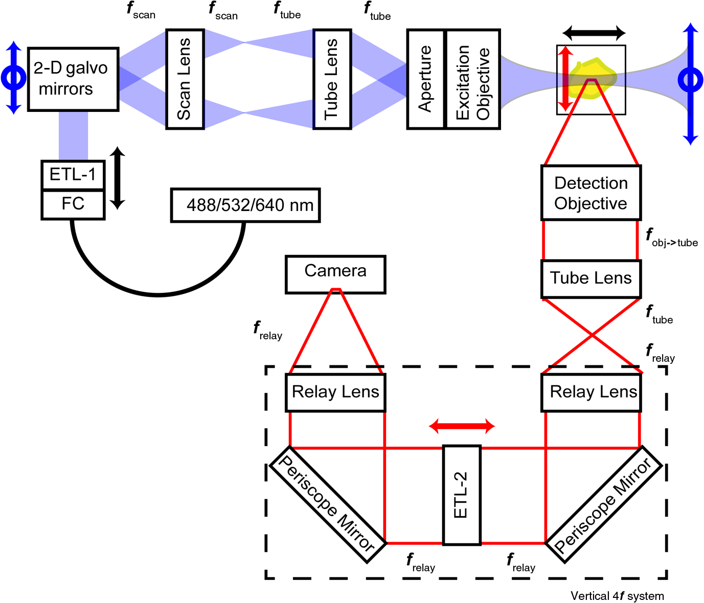 A 3-D printed imaging chamber, with glued #1 quartz coverslips (SPI Supplies 01019T-AB), was mounted to a manual rotation stage (Thorlabs PR01) and centered at the focal length of both the excitation and detection objectives (DOs), so the full range of excitation beam scanning was available (). An automated micrometer-driven stage controlled using OpenStage hardware and software was utilized for sample positioning and tiling.44 This stage positioned a sample rotation stage/sample mount consisting of an Arduino Uno controlled stepper motor (Sparkfun DEV-11021, Sparkfun ROB-09238) and rigid mounted pipette tip within the imaging chamber. The detection arm accommodated a NA 0.13 17.2-mm WD (Nikon MRH00041) or NA 0.28 33.5-mm WD (Edmund Optics 59-877) DO using a nonrotating translatable objective mount (Thorlabs SM1NR1). A tube lens (Nikon MXA22018), adjustable periscope mirror (Thorlabs BB1-E02), and electrotunable lens (ETL-2 – Optotune EL-16-40-TC) were placed at the first focal point of a system (Thorlabs AC254-300-A). An adjustable periscope mirror (Thorlabs BB1-E02), automated filter wheel (Thorlabs FW102C), and sCMOS camera (Hamamatsu C11440-22CU) completed the detection optics. ETL-2 was placed in a configuration to allow the focus to be swept without changing telecentricity. To generate images the scanning mirror corresponding to the focal plane (fast-axis) was swept once per acquisition. The second scanning mirror positioned the light sheet along the detection axis. ETL-2 positioned the focal plane of camera at the axial location of the light sheet. ETL-1 optimized the alignment of each laser source, enabling fine tuning of the excitation arm focus within the sample. These values were user determined at multiple image planes throughout the sample. The full table of axial mirror, ETL-1, and ETL-2 values were then built using linear interpolation. This technique allowed the sample to stay immobile during volumetric imaging. For all images in this work, fluorescence was collected with either the NA 0.13 or NA 0.28 DO. This yielded in-plane pixel sizes of 1.625 or and axial step sizes of 3.5 or , respectively. A manually adjustable pinhole was utilized to limit the NA of the excitation objective to adjust the Rayleigh length to best match the imaging area. This yielded a Gaussian width of for the DO and for the DO. Volumetric images of varying total sizes at orientations parallel or perpendicular to the optic nerve were acquired for each retina. The orientation that best visualized the vasculature was chosen for image analysis. 2.9.Two-Dimensional Fluorescent Image QuantificationAll 20× images were imported into Angiotool for automated network tracing.16 Analysis parameters were visually modified for accurate skeletonization. Controls were set to a low threshold of 15, high threshold of 255, and vessel diameter of 15 and to fill holes at 2000. Output metrics included vessel percentage area, total number of junctions, junction density, total vessel length, average vessel length, total number of endpoints, and mean lacunarity. Statistical analysis was performed in Graphpad PRISM using an ANOVA test. Additionally, the binary image produced by Angiotool was analyzed using 2-D Sholl analysis in FIJI.39,41 The number of intersections as a function of radius was normalized by the area of the circle. The resulting Sholl curves were then integrated using trapezoidal integration with unit spacing in MATLAB®. Statistical analysis was performed in MATLAB® using a Kruskal–Wallis test. 2.10.Two-Dimensional Fluorescent Optically Sectioned Image QuantificationOptically sectioned images of retina flat mounts were analyzed using FIJI and Vaa3D.32,36 Images were filtered using a multiscale adaptive enhancement filter.30 Semiautomated network tracing was carried out on filtered images using APP-2.0.31 The resulting network trace was used to mask the retinal vasculature into a binary image. The binary image was analyzed using 2-D Sholl analysis for each image plane in FIJI.39,41 The number of intersections as a function of radius was normalized by the area of the circle for each focal plane. The resulting Sholl curves were then integrated using trapezoidal integration with unit spacing in MATLAB®. Statistical analysis was performed in MATLAB® using a Kruskal–Wallis test. 2.11.Three-Dimensional Fluorescent Image Network Quantification PipelineVolumetric images of intact retinas were analyzed in Vaa3D.36 Raw images were filtered using a multiscale adaptive enhancement filter.34 Semiautomated network tracing was carried out on filtered images using APP-2.0.35 The resulting network trace was used to mask the retinal vasculature into a binary image. The binary image was analyzed using 3-D Sholl analysis in FIJI.39,41 The number of intersections as a function of radius was normalized by the surface area of the sphere. The resulting Sholl curves were then integrated using trapezoidal integration with unit spacing in MATLAB®. Statistical analysis was performed in MATLAB® using a Kruskal–Wallis test. 3.Results3.1.Superficial Vascular Plexus was Disturbed at P7 in Continuous Hyperoxia Exposure ModelP7 RA control retinas displayed dense and consistent vascular distributions with narrow avascular zones at the retinal periphery [Fig. 3(a)]. In contrast, P7 HO flat mounts showed simplified vessel branching and decreased vessel concentration throughout the primary plexus, with large avascular zones at the retinal periphery [Fig. 3(b)]. Fig. 3Representative tiled and segmented epifluorescence images of P7 retinal flat mounts. (a) Control retinal flat mounts show normal vascular development and (b) HO retinal flat mounts show simplified and less expansive vasculature (shaded red area and red asterisk). Pixel size of and total image size of . Raw images segmented using automatically determined global threshold and Otsu algorithm in FIJI. 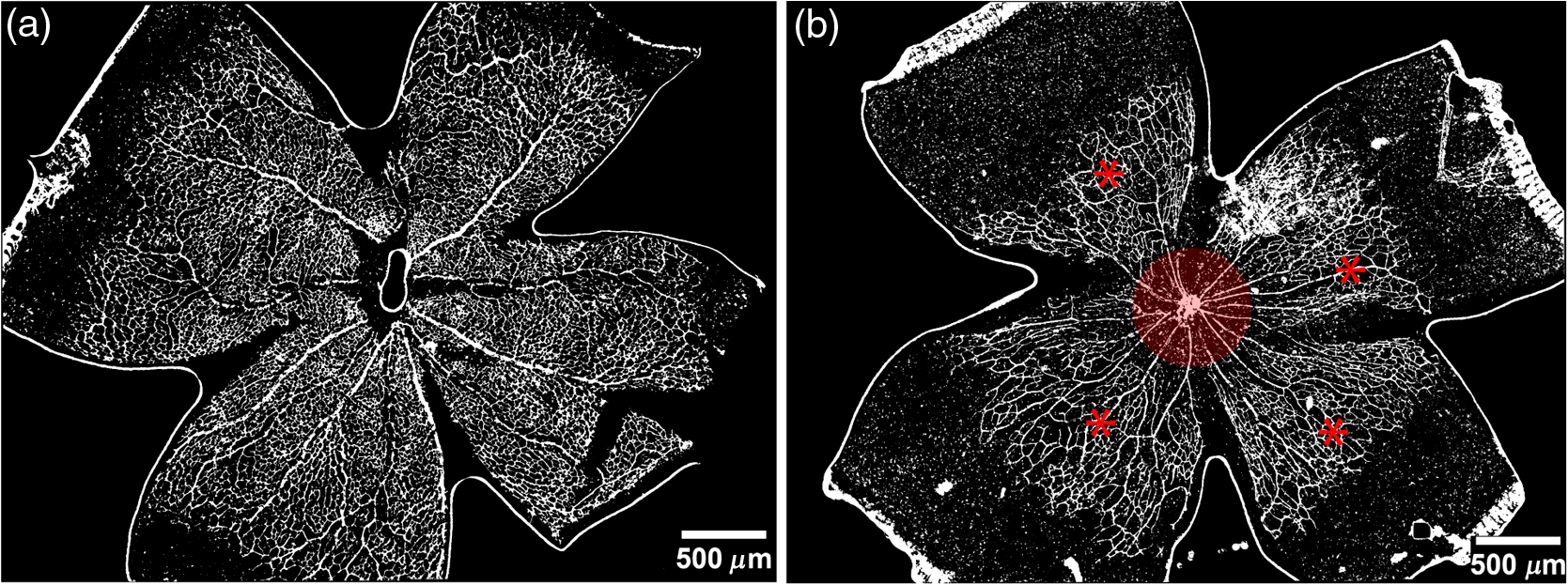 To better visualize the 3-D structure of the developing rat retinal vasculature, we imaged intact retinas using DSLM (Fig. 4, Videos 1 and 2). This imaging method offered two advantages over traditional flat mount preparations. The native structure of the eye was better preserved because the retina was not physically altered, and volumetric imaging proceeded rapidly, at to 500 ms per image plane. For Figs. 4(a) and 4(b), the image acquisition required roughly 5 min. For the multiple overlapping images that comprise Figs. 4(c) and 4(d), image acquisition required roughly 30 min. In comparison, acquisition of a similar volume in a retinal flat mount using a wide-field deconvolution microscope or a confocal microscope required nearly 10 h. Fig. 4Three-dimensional renderings of DSLM imaging of intact retinas. (a) Low-magnification 3-D rendering of P14 rat retinas. In-plane pixel size of and axial step of . Total imaging volume . (Video 1, MP4, 2.5 MB [URL: http://dx.doi.org/10.1117/1.JBO.22.7.076011.1]) (b) Cross-sectional image of (a). In-plane pixel size of and axial step of . Total imaging volume . (c) High-resolution 3-D image of intact P7 retina. In-plane pixel size of and axial step of . Total imaging volume . (Video 2, MP4, 3.7 MB [URL: http://dx.doi.org/10.1117/1.JBO.22.7.076011.2]) (d) Zoomed area showing intact primary plexus (left), vertical sprouts (middle), secondary plexus (right), and choroid vasculature (far right). In-plane pixel size of and axial step of . Total imaging volume .  Individual image planes contained within volumetric images showed the presence of the choroid layer of vasculature, as well as the primary plexus and the secondary plexus found at the deepest portion of the retina. Connections were observed between the two plexuses in control retinas, indicating the presence of vertical sprouts [Fig. 5(a)]. In the HO retinas, the strongest fluorescent signal was found at the site of the primary plexus. This appeared as dense fluorescence, suggesting an abnormal vascular distribution [Fig. 5(b)]. Additionally, the choroids of the HO retinas were consistently deformed compared to those of the control retinas [Fig. 5(b)]. Fig. 5Representative individual image planes from volumetric DSLM images of P7 intact retinas. (a) P7 control retinas show normal development of the (1) primary plexus, (2) vertical sprouts, (3) secondary vascular plexus, and (4) smooth choroid. (b) P7 HO retinas show a chaotic (1) primary plexus, lack of vertical sprouts and secondary plexus, and (4) distorted choroid. Individual image planes isolated from full axial image stacks with a pixel size of . 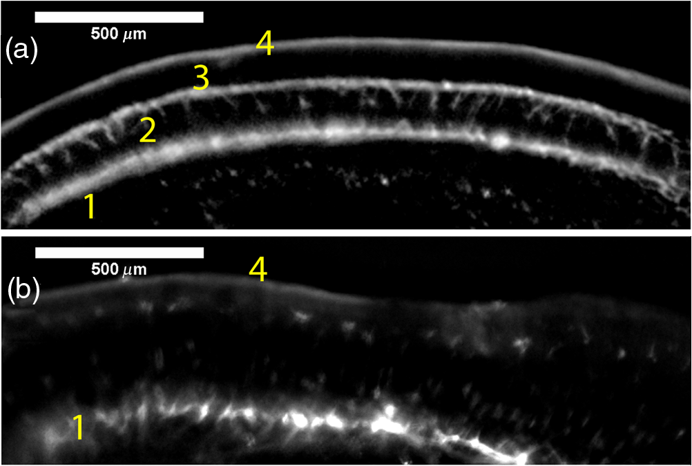 3.2.Secondary Vascular Plexus Remained Disorganized in P14 RetinasVascular development at P14 was more robust compared with P7 in both control and HO retinas. Relative to control P14 retinas [Fig. 6(a)], P14 HO retinas demonstrated reduced vascular complexity surrounding the optic nerve and larger avascular zones at the retinal periphery [Fig. 6(b)]. P14 DSLM images also showed more robust vasculature compared with P7 images. Control P14 retinas demonstrated more vertical sprouts and more organized primary and secondary plexuses [Fig. 7(a)]. HO P14 retinas demonstrated a strong fluorescent signal in the primary plexus, but they appeared disorganized compared to control retinas. [Fig. 7(b)]. Fig. 6Representative tiled and segmented epifluorescence images of P14 retinal flat mounts. (a) P14 control retinal flat mounts show normal vascular development and (b) P14 HO retinal flat mounts show some decrease in primary plexus development, particularly surrounding the optic nerve (shaded red area and red asterisks). Pixel size of and total image size of . Raw images segmented using automatically determined global threshold and Otsu algorithm in FIJI. 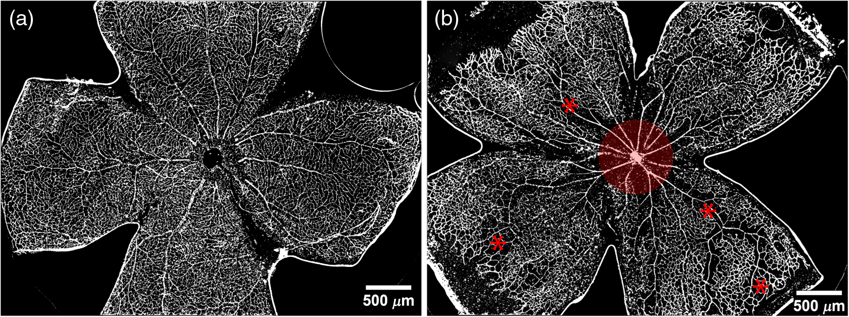 Fig. 7Representative individual image planes from volumetric DSLM images of intact P14 retinas. (a) P14 control retinas show a fully developed (1) primary and (3) secondary vascular plexus, as well as (2) vertical sprouts with a (4) smooth choroid. (b) P14 HO retinas show clear staining for a developed (1) primary plexus. However, there is diffuse staining, indicating disorganized (2) vertical sprouts, lack of a secondary plexus, and (4) distorted choroid. Individual image planes isolated from full axial image stacks with a pixel size of . 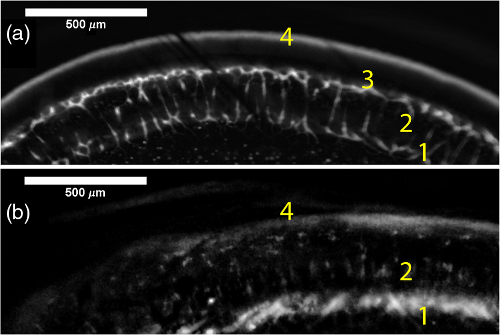 To verify these findings, we performed optical sectioning of retinal flat mounts utilizing a high NA objective, epifluorescence, and computational deconvolution. Figure 8 shows an axial montage of the vascular network isolated from a large-scale epifluorescence image ( image areas per retina) of control and HO retinas at P7. Vertical sprouts and secondary plexuses were missing from HO retinas [red arrows note sprouts in Fig. 8(a)]. Fig. 8Representative cross-sections from deconvolved epifluorescence images of P7 retinal flat mounts. (a) P7 control retinas show the beginning of a highly organized network sprouting from the primary plexus. Red arrows mark vertical sprouts that are found in multiple axial planes in P7 control retinas. (b) P7 HO retinas show little evidence of vertical sprouts. No continuous vertical sprouts are found in P7 HO retinas in this area. This result holds throughout the entire retina. 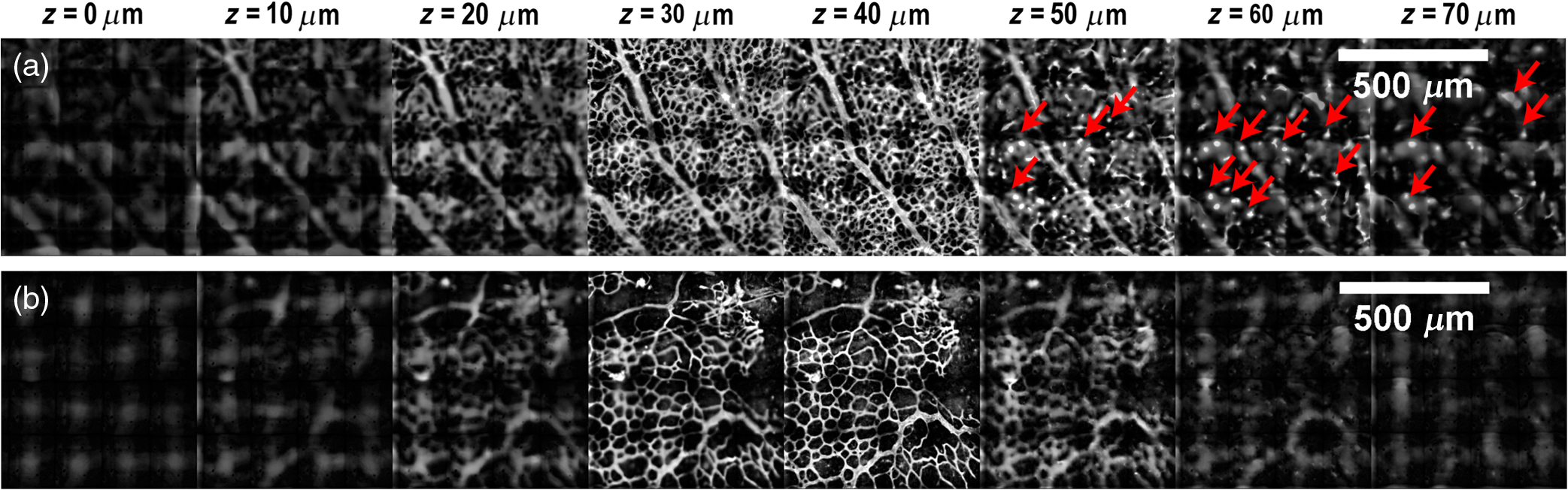 3.3.Quantification of Vascular Complexity Using Traditional Network TracingWe used Angiotool software to quantify the differences in the primary plexus between control and continuous HO exposed retinas at the two time points used in this study. Angiotool measures morphometric and spatial parameters of vascularity through network tracing [Fig. 9(a)]. We utilized the total vessel length, junction density, and mean lacunarity tools for assessment of the images (Figs. 2 and 5).16 We observed a significant decrease in total vessel length and junction density between control and HO P7 retinas [Figs. 9(b) and 9(c)]. This lack of vascular complexity appeared to resolve by P14, with no statistical difference between the two study groups at that time point. Inversely, we saw an increase in avascular space measured by mean lacunarity at P7 in HO relative to controls [Fig. 9(d)]. Again, there was no statistical difference between mean lacunarity in the two groups by P14. Angiotool was designed to measure morphometric and spatial parameters of vascularity in two dimensions through skeletonization and feature extraction. Because the algorithm does not consider axial network connections and requires high signal-to-noise for feature identification, it was not applied to 3-D and volumetric images. Fig. 9Angiotool analysis applied to retina vascular networks. (a) Example of Angiotool network tracing. (b) Total vessel length decreased in HO eyes at P7, resolves by P14. (c) Junction density decreased in HO eyes at P7, resolves by P14. (d) Mean lacunarity increased in HO eyes at P7, resolves by P14. * denotes using ANOVA test. All data are .  3.4.Quantification of Vascular Complexity Using Sholl AnalysisWe conducted Sholl analysis to quantify the variations in vascular distribution between control and HO retinas. Previously used to quantify characteristics of dendritic processes branching off neuronal cell bodies, Sholl analysis examines the number of branches that intersect concentric circles (retinal flat mounts) or spheres (intact retinas) of increasing radii around the cell body or central focal point of the image area (Fig. 10).38,39 Fig. 10Sholl analysis applied to retinal vascular networks. Schematic of Sholl analysis applied to retinal flat mount. Starting from the center of the retina, equally spaced concentric circles (shaded red) are superimposed on a segmented image of the retinal flat mount. Along each circle, the number of intersections with the vascular network is counted (inset: yellow star along red lines). This provides a measure of the vascular network complexity as a function of radial distance from the center.  Using this method, we observed an initial decrease in vascular branching in HO P7 retinas compared with those of the control [Figs. 11(a) and 11(c)]. This was consistent with our observations using DSLM and intact retinas in which there was a reduction or complete absence of the secondary plexus in HO retinas. Three-dimensional Sholl analysis applied to intact P14 retinas captured this observation while 2-D Sholl analysis applied to P14 retinal flat mounts failed to account for the lack of secondary plexus [Figs. 11(b) and 11(d)]. We utilized the “integrated” Sholl metric by taking the integral of the area under the Sholl analysis curve to calculate an approximate value of the total number of vascular network intersections (Fig. 12).4 This simple metric captures changes in 3-D vascular structure of intact retinas, providing a methodology to rapidly quantify the full vascular development of the retina. Fig. 11Sholl analysis results. Mean (solid) and standard deviation (shaded) of normalized Sholl curves for control (black) and HO (red). (a) P7 retinal flat mounts, (b) P14 retinal flat mounts, (c) intact P7 retinas, and (d) intact P14 retinas ( for each group). There is a clear difference in vascular complexity at P7 for both flat mount and intact retinas. However, at P14, there is no clear difference in retinal flat mounts and a less pronounced difference in intact retinas. 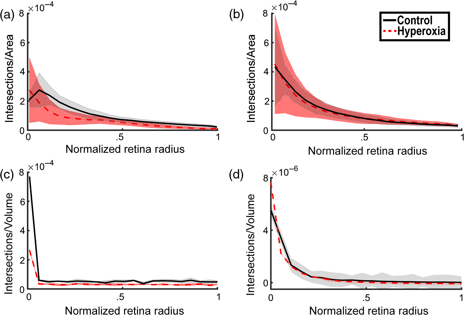 Fig. 12Box and whisker plots of integrated normalized Sholl metric. The Sholl metric is calculated for (a) retinal flat mounts and (b) intact retinas by integrating the area under each normalized curve. The metric is not comparable between flat mounts and intact retinas due to different normalizations (area versus volume). At P7, RA and HO flat mounts and intact retina vascular networks are statistically different (, Kruskal–Wallis test, ). At P14, RA and HO flat mounts are not statistically different (, Kruskal–Wallis test) while RA and HO intact retinas are (, Kruskal–Wallis test, ). 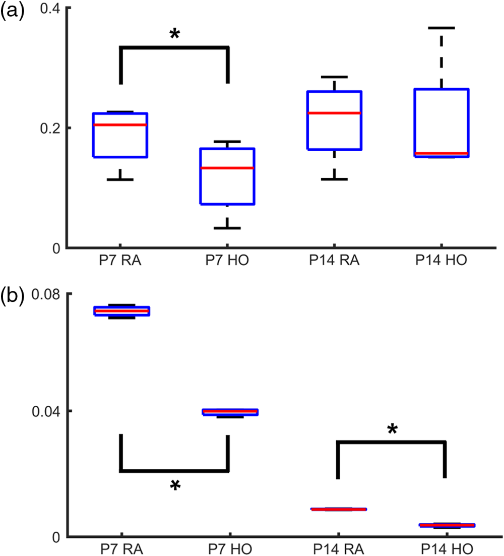 4.DiscussionIn this study, we used a continuous HO exposure model to produce significant vascular abnormality in rat retinas. We quantified these abnormalities by comparing control retinas to HO retinas using multiple imaging modalities. These data were collected using two distinct techniques in microscopy and image analysis; epifluorescence imaging with Angiotool and Sholl analysis, as well as DSLM imaging with Sholl analysis. The two methods were compared based on retinal distortion due to sample preparation, imaging depth, and vascular network quantification. At P7, both imaging techniques showed that HO exposure caused stunted vessel growth in the central retina and the cessation of normal radial vessel growth in the primary plexus. DSLM images also displayed an absent secondary plexus in the HO retinas. Previous studies have shown that HO during postnatal retinal development causes downregulation of hypoxia inducible factor, preventing the release of vascular endothelial growth factor and insulin-like growth factor and the formation of a normal retinal vascular plexus.45,46 Because sprouting from the primary plexus toward the secondary plexus appeared delayed, we speculate that oxygen exposure may have negatively impacted other cell types driving angiogenesis. The exact molecular mechanisms that control this sprouting into the secondary plexus are not well understood, making this a potential area of future study using these techniques.47,48 At P14, we observed recovery of the primary vascular plexus in HO retinas with both imaging techniques but saw that the secondary plexus was not always restored in the DSLM images. This suggests that compensatory signaling, possibly initiated by an increasingly avascular retina or hyperoxia suppresses development of the deeper vasculature.49 Traditionally, retinal vascular networks are quantified based on features detectable in fluorescent images of the primary plexus. These quantifications involve morphometric measurements, such as the number of junctions, branch points, vessel length, and overall vessel density. These images come from flat mounts, which require significant sample manipulation and therefore may compromise biological data. Traditional network tracing programs such as Angiotool are designed for 2-D image analysis, limiting their capacity to measure vascular development below the primary plexus.16 For comparison, we employed DSLM to visualize the locations of the primary and secondary plexus, separated by an intermediary layer (Fig. 6). This allowed for visualization of all layers of the retinal vasculature in the native confirmations. Not only did DSLM provide more accurate and robust data, but we gained additional spatial information regarding pathological vascularization. In control retinas, vertical sprouts were easily visualized in the intermediary layer at P7 and P14. In HO retinas, we observed an absence of intermediate sprouting at P7 and subsequent recovery by P14. The use of air-immersion microscope objectives in our DSLM led to a spherical aberration when imaging optically cleared tissue immersed in a refractive index matching solution.33,50 While this aberration minimally disrupts imaging of the vascular system, further investigations of molecular mechanisms or single-cell identification will be complicated by aberrations. Future work to integrate refractive index corrected optics (narrow field of view) or computational fusion/deconvolution methods (multiple image orientations and intensive computation) will increase imaging time but reduce optical aberrations.33,51,52 We show that Sholl analysis captures the complexity of the vascular network in two- and three-dimensions. Integrating the resulting Sholl curves provides a simplified metric that can be utilized to rapidly compare retinal vasculature without morphometric measurements. Adapting Sholl analysis to 3-D confocal or two-photon imaging of retinal flat mounts will require careful consideration of the correct normalization procedure. 5.ConclusionAs treatments to promote physiologic retinal vascular development are evaluated, 3-D imaging techniques that are compatible with cellular and protein-specific staining are highly sought after. DSLM imaging techniques provide a promising approach to studying the molecular mechanisms involved in the regulation of angiogenesis. Most studies of retinal vascular development focus on the superficial primary vascular plexus, whereas the intermediate and deep secondary plexuses have been less explored. Mapping the entire 3-D, interconnected network can comprehensively capture the complex nature of vascular development in a way that current methods cannot. When combined with optical tissue clearing, this imaging methodology allows for quantification of protein signaling and individual cell type. This will enable future studies to map the 3-D distribution of signaling fronts and vascular structure within intact retinas. Reducing the complexity of high-dimensional datasets into meaningful metrics and statistical measures to test hypotheses also remains an ongoing challenge. Here, we have shown that Sholl analysis can be readily adapted to generate an integrated normalized Sholl metric that provides an easy way to compare the measure of vascular complexity in both retinal flat mounts and intact retinas. AcknowledgmentsWe thank Dr. Julie Siegenthaler for helpful discussions regarding rodent models of retinal development. J.N.S. and D.P.S. acknowledge the CU Denver College of Liberal Arts and Sciences start-up funding and National Institutes of Health (NIH) National Institute on Aging AG053690. T.M.N., G.J.S., and S.H.A. acknowledge funding from NIH National Heart, Lung, and Blood Institute HL68702. ReferencesM. Fruttiger,
“Development of the retinal vasculature,”
Angiogenesis, 10
(2), 77
–88
(2007). http://dx.doi.org/10.1007/s10456-007-9065-1 Google Scholar
T. L. Terry,
“Retrolental fibroplasia in the premature infant: V. Further studies on fibroplastic overgrowth of the persistent tunica vasculosa lentis,”
Trans. Am. Ophthalmol. Soc., 42 383
–396
(1944). TAOSAT 0065-9533 Google Scholar
J. Chen and L. E. H. Smith,
“Retinopathy of prematurity,”
Angiogenesis, 10
(2), 133
–140
(2007). http://dx.doi.org/10.1007/s10456-007-9066-0 Google Scholar
R. D. Jager, W. F. Mieler and J. W. Miller,
“Age-related macular degeneration,”
N. Engl. J. Med., 358
(24), 2606
–2617
(2008). http://dx.doi.org/10.1056/NEJMra0801537 NEJMAG 0028-4793 Google Scholar
M. I. Dorrell and M. Friedlander,
“Mechanisms of endothelial cell guidance and vascular patterning in the developing mouse retina,”
Prog. Retinal Eye Res., 25
(3), 277
–295
(2006). http://dx.doi.org/10.1016/j.preteyeres.2006.01.001 PRTRES 1350-9462 Google Scholar
L. Smith et al.,
“Oxygen-induced retinopathy in the mouse,”
Invest. Ophthalmol. Vis. Sci., 35
(1), 101
–111
(1994). IOVSDA 0146-0404 Google Scholar
J. S. Penn, B. L. Tolman and L. A. Lowery,
“Variable oxygen exposure causes preretinal neovascularization in the newborn rat,”
Invest. Ophthalmol. Vis. Sci., 34
(3), 576
–585
(1993). IOVSDA 0146-0404 Google Scholar
J. M. Barnett, S. E. Yanni and J. S. Penn,
“The development of the rat model of retinopathy of prematurity,”
Doc. Ophthalmol., 120
(1), 3
–12
(2010). http://dx.doi.org/10.1007/s10633-009-9180-y Google Scholar
A. Stahl et al.,
“The mouse retina as an angiogenesis model,”
Invest. Opthalmol. Vis. Sci., 51
(6), 2813
(2010). http://dx.doi.org/10.1167/iovs.10-5176 Google Scholar
X. Gu et al.,
“Effects of sustained hyperoxia on revascularization in experimental retinopathy of prematurity,”
Invest. Ophthalmol. Vis. Sci., 43
(2), 496
–502
(2002). IOVSDA 0146-0404 Google Scholar
K. M. Connor et al.,
“Quantification of oxygen-induced retinopathy in the mouse: a model of vessel loss, vessel regrowth and pathological angiogenesis,”
Nat. Protoc., 4
(11), 1565
–1573
(2009). http://dx.doi.org/10.1038/nprot.2009.187 1754-2189 Google Scholar
J. M. Furtado et al.,
“Imaging retinal vascular changes in the mouse model of oxygen-induced retinopathy,”
Transl. Vision. Sci. Technol., 1
(2), 5
(2012). http://dx.doi.org/10.1167/tvst.1.2.5 Google Scholar
Y. Chikaraishi, M. Shimazawa and H. Hara,
“New quantitative analysis, using high-resolution images, of oxygen-induced retinal neovascularization in mice,”
Exp. Eye Res., 84
(3), 529
–536
(2007). http://dx.doi.org/10.1016/j.exer.2006.11.007 EXERA6 0014-4835 Google Scholar
J. Browning, C. K. Wylie and G. Gole,
“Quantification of oxygen-induced retinopathy in the mouse,”
Invest. Ophthalmol. Visual Sci., 38
(6), 1168
–1174
(1997). IOVSDA 0146-0404 Google Scholar
M. B. Vickerman et al.,
“VESGEN 2D: automated, user-interactive software for quantification and mapping of angiogenic and lymphangiogenic trees and networks,”
Anat. Rec., 292
(3), 320
–332
(2009). http://dx.doi.org/10.1002/ar.v292:3 Google Scholar
E. Zudaire et al.,
“A computational tool for quantitative analysis of vascular networks,”
PLoS One, 6
(11), e27385
(2011). http://dx.doi.org/10.1371/journal.pone.0027385 POLNCL 1932-6203 Google Scholar
H. Hammer et al.,
“Scattering properties of the retina and the choroids determined from OCT-A-scans,”
Int. Ophthalmol., 23
(4–6), 291
–295
(2001). http://dx.doi.org/10.1023/A:1014430009122 Google Scholar
H. Luan et al.,
“Retinal thickness and subnormal retinal oxygenation response in experimental diabetic retinopathy,”
Invest. Ophthalmol. Visual Sci., 47
(1), 320
–328
(2006). http://dx.doi.org/10.1167/iovs.05-0272 IOVSDA 0146-0404 Google Scholar
D. K. Sardar et al.,
“Optical absorption and scattering of bovine cornea, lens and retina in the visible region,”
Lasers Med. Sci., 24
(6), 839
–847
(2009). http://dx.doi.org/10.1007/s10103-009-0677-0 Google Scholar
Y. Wang et al.,
“Norrin/Frizzled4 signaling in retinal vascular development and blood brain barrier plasticity,”
Cell, 151
(6), 1332
–1344
(2012). http://dx.doi.org/10.1016/j.cell.2012.10.042 CELLB5 0092-8674 Google Scholar
F. Milde et al.,
“The mouse retina in 3D: quantification of vascular growth and remodeling,”
Integr. Biol., 5
(12), 1426
–1438
(2013). http://dx.doi.org/10.1039/c3ib40085a 1757-9708 Google Scholar
X. Ye, Y. Wang and J. Nathans,
“The Norrin/Frizzled4 signaling pathway in retinal vascular development and disease,”
Trends Mol. Med., 16
(9), 417
–425
(2010). http://dx.doi.org/10.1016/j.molmed.2010.07.003 Google Scholar
B. R. Masters and M. Böhnke,
“Three-dimensional confocal microscopy of the living human eye,”
Annu. Rev. Biomed. Eng., 4
(1), 69
–91
(2002). http://dx.doi.org/10.1146/annurev.bioeng.4.092701.132001 ARBEF7 1523-9829 Google Scholar
A. G. Podoleanu et al.,
“Three dimensional OCT images from retina and skin,”
Opt. Express, 7
(9), 292
(2000). http://dx.doi.org/10.1364/OE.7.000292 OPEXFF 1094-4087 Google Scholar
C. K. Hitzenberger et al.,
“Three-dimensional imaging of the human retina by high-speed optical coherence tomography,”
Opt. Express, 11
(21), 2753
(2003). http://dx.doi.org/10.1364/OE.11.002753 OPEXFF 1094-4087 Google Scholar
B. A. Nemet, V. Nikolenko and R. Yuste,
“Second harmonic imaging of membrane potential of neurons with retinal,”
J. Biomed. Opt., 9
(5), 873
–881
(2004). http://dx.doi.org/10.1117/1.1783353 JBOPFO 1083-3668 Google Scholar
O. Masihzadeh et al.,
“Third harmonic generation microscopy of a mouse retina,”
Mol. Vision, 21 538
–547
(2015). Google Scholar
U.-D. Braumann et al.,
“Large histological serial sections for computational tissue volume reconstruction,”
Methods Inf. Med., 46
(5), 614
–622
(2007). Google Scholar
B. Yang et al.,
“Single-cell phenotyping within transparent intact tissue through whole-body clearing,”
Cell, 158
(4), 945
–958
(2014). http://dx.doi.org/10.1016/j.cell.2014.07.017 CELLB5 0092-8674 Google Scholar
J. B. Treweek et al.,
“Whole-body tissue stabilization and selective extractions via tissue-hydrogel hybrids for high-resolution intact circuit mapping and phenotyping,”
Nat. Protoc., 10
(11), 1860
–1896
(2015). http://dx.doi.org/10.1038/nprot.2015.122 1754-2189 Google Scholar
P. J. Keller and E. H. Stelzer,
“Quantitative in vivo imaging of entire embryos with digital scanned laser light sheet fluorescence microscopy,”
Curr. Opin. Neurobiol., 18
(6), 624
–632
(2008). http://dx.doi.org/10.1016/j.conb.2009.03.008 COPUEN 0959-4388 Google Scholar
J. Huisken et al.,
“Optical sectioning deep inside live embryos by selective plane illumination microscopy,”
Science, 305
(5686), 1007
–1009
(2004). http://dx.doi.org/10.1126/science.1100035 SCIEAS 0036-8075 Google Scholar
R. Tomer et al.,
“Advanced CLARITY for rapid and high-resolution imaging of intact tissues,”
Nat. Protoc., 9
(7), 1682
–1697
(2014). http://dx.doi.org/10.1038/nprot.2014.123 1754-2189 Google Scholar
Z. Zhou et al.,
“Adaptive image enhancement for tracing 3D morphologies of neurons and brain vasculatures,”
Neuroinformatics, 13
(2), 153
–166
(2015). http://dx.doi.org/10.1007/s12021-014-9249-y 1539-2791 Google Scholar
H. Xiao and H. Peng,
“APP2: automatic tracing of 3D neuron morphology based on hierarchical pruning of a gray-weighted image distance-tree,”
Bioinformatics, 29
(11), 1448
–1454
(2013). http://dx.doi.org/10.1093/bioinformatics/btt170 BOINFP 1367-4803 Google Scholar
H. Peng et al.,
“Extensible visualization and analysis for multidimensional images using Vaa3D,”
Nat. Protoc., 9
(1), 193
–208
(2014). http://dx.doi.org/10.1038/nprot.2014.011 1754-2189 Google Scholar
H. Peng et al.,
“Automatic tracing of ultra-volumes of neuronal images,”
Nat. Methods, 14
(4), 332
–333
(2017). http://dx.doi.org/10.1038/nmeth.4233 1548-7091 Google Scholar
D. A. Sholl,
“Dendritic organization in the neurons of the visual and motor cortices of the cat,”
J. Anat., 87
(4), 387
–406
(1953). JOANAY 0021-8782 Google Scholar
T. A. Ferreira et al.,
“Neuronal morphometry directly from bitmap images,”
Nat. Methods, 11
(10), 982
–984
(2014). http://dx.doi.org/10.1038/nmeth.3125 1548-7091 Google Scholar
M. A. Bruce and M. J. Butte,
“Real-time GPU-based 3D deconvolution,”
Opt. Express, 21
(4), 4766
–4773
(2013). http://dx.doi.org/10.1364/OE.21.004766 OPEXFF 1094-4087 Google Scholar
J. Schindelin et al.,
“Fiji: an open-source platform for biological-image analysis,”
Nat. Methods, 9
(7), 676
–682
(2012). http://dx.doi.org/10.1038/nmeth.2019 1548-7091 Google Scholar
S. Preibisch, S. Saalfeld and P. Tomancak,
“Globally optimal stitching of tiled 3D microscopic image acquisitions,”
Bioinformatics, 25
(11), 1463
–1465
(2009). http://dx.doi.org/10.1093/bioinformatics/btp184 BOINFP 1367-4803 Google Scholar
D. Ryan et al.,
“Automatic and adaptive heterogeneous refractive index compensation for light-sheet microscopy,”
Nat. Commun., Google Scholar
R. A. A. Campbell, R. W. Eifert and G. C. Turner,
“Openstage: a low-cost motorized microscope stage with sub-micron positioning accuracy,”
PLoS One, 9
(2), e88977
(2014). http://dx.doi.org/10.1371/journal.pone.0088977 POLNCL 1932-6203 Google Scholar
C. Lofqvist et al.,
“IGFBP3 suppresses retinopathy through suppression of oxygen-induced vessel loss and promotion of vascular regrowth,”
Proc. Natl. Acad. Sci. U. S. A., 104
(25), 10589
–10594
(2007). http://dx.doi.org/10.1073/pnas.0702031104 Google Scholar
A. Hellstrom,
“Low IGF-I suppresses VEGF-survival signaling in retinal endothelial cells: direct correlation with clinical retinoapthy of prematurity,”
Proc. Natl. Acad. Sci. U. S. A., 98
(10), 5804
–5808
(2001). Google Scholar
R. F. Gariano and T. W. Gardner,
“Retinal angiogenesis in development and disease,”
Nature, 438
(7070), 960
–966
(2004). http://dx.doi.org/10.1038/nature04482 Google Scholar
R. F. Gariano,
“Special features of human retinal angiogenesis,”
Eye, 24
(3), 401
–407
(2010). http://dx.doi.org/10.1038/eye.2009.324 12ZYAS 0950-222X Google Scholar
M. McCloskey et al.,
“Anti-VEGF antibody leads to later atypical intravitreous neovascularization and activation of angiogenic pathways in a rat model of retinopathy of Prematurity Anti-VEGF antibody in ROP model,”
Invest. Ophthalmol. Visual Sci., 54
(3), 2020
–2026
(2013). http://dx.doi.org/10.1167/iovs.13-11625 IOVSDA 0146-0404 Google Scholar
L. Silvestri, L. Sacconi and F. S. Pavone,
“Correcting spherical aberrations in confocal light sheet microscopy: a theoretical study,”
Microsc. Res. Tech., 77
(7), 483
–491
(2014). http://dx.doi.org/10.1002/jemt.v77.7 MRTEEO 1059-910X Google Scholar
R. Tomer et al.,
“SPED light sheet microscopy: fast mapping of biological system structure and function,”
Cell, 163
(7), 1796
–1806
(2015). http://dx.doi.org/10.1016/j.cell.2015.11.061 CELLB5 0092-8674 Google Scholar
S. Preibisch et al.,
“Efficient Bayesian-based multiview deconvolution,”
Nat. Methods, 11
(6), 645
–648
(2014). http://dx.doi.org/10.1038/nmeth.2929 1548-7091 Google Scholar
BiographyDouglas P. Shepherd is an assistant professor at the University of Colorado Denver. He received his BS degree in physics from the University of California, Santa Barbara, in 2003 and his PhD in physics from Colorado State University in 2013. His current research interests include single-molecule biophysics and light-sheet microscopy of optically cleared tissue. |


