Automated framework for intraretinal cystoid macular edema segmentation in three-dimensional optical coherence tomography images with macular hole

Weifang Zhu; Li Zhang; Fei Shi; Dehui Xiang; Lirong Wang; Jingyun Guo; Xiaoling Yang; Haoyu Chen; Xinjian Chen

doi:10.1117/1.JBO.22.7.076014

21 July 2017 Automated framework for intraretinal cystoid macular edema segmentation in three-dimensional optical coherence tomography images with macular hole

Weifang Zhu, Li Zhang, Fei Shi, Dehui Xiang, Lirong Wang, Jingyun Guo, Xiaoling Yang, Haoyu Chen, Xinjian Chen

Author Affiliations +

Journal of Biomedical Optics, Vol. 22, Issue 7, 076014 (July 2017). https://doi.org/10.1117/1.JBO.22.7.076014

Abstract

Cystoid macular edema (CME) and macular hole (MH) are the leading causes for visual loss in retinal diseases. The volume of the CMEs can be an accurate predictor for visual prognosis. This paper presents an automatic method to segment the CMEs from the abnormal retina with coexistence of MH in three-dimensional-optical coherence tomography images. The proposed framework consists of preprocessing and CMEs segmentation. The preprocessing part includes denoising, intraretinal layers segmentation and flattening, and MH and vessel silhouettes exclusion. In the CMEs segmentation, a three-step strategy is applied. First, an AdaBoost classifier trained with 57 features is employed to generate the initialization results. Second, an automated shape-constrained graph cut algorithm is applied to obtain the refined results. Finally, cyst area information is used to remove false positives (FPs). The method was evaluated on 19 eyes with coexistence of CMEs and MH from 18 subjects. The true positive volume fraction, FP volume fraction, dice similarity coefficient, and accuracy rate for CMEs segmentation were 81.0%±7.8%, 0.80%±0.63%, 80.9%±5.7%, and 99.7%±0.1%, respectively.

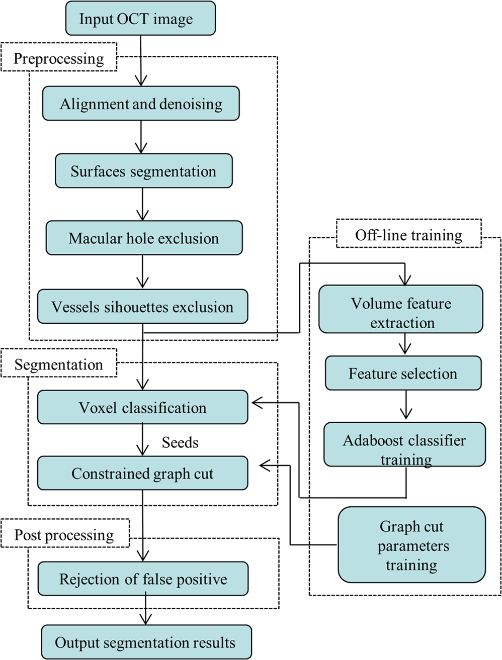
1. Introduction

Optical coherence tomography (OCT) is becoming a mainstay in ophthalmology as a noninvasive imaging technique for human retina.¹^–⁴ OCT has been widely used in the diagnosis of ocular diseases, such as macular edema (ME), macular hole (MH), glaucoma, etc. The macula is located near the center of the retina and is responsible for central, high-resolution, and color vision. Some acute maculopathies may lead to the loss of central vision and even blindness.⁵ MH is a full-thickness defect of neurosensory retina involving the anatomic fovea which severely affects central visual acuity.⁶ The overall incidence of MH is $\sim 3.3$ cases in 1000 in the United States.⁷ MH often progresses gradually and is common in people of age 60 and over.⁸ A person with MH may notice a slight distortion or blurriness in straight-ahead vision. Cystoid macular edema (CME) occurs in a wide variety of ocular diseases, such as diabetic retinopathy, intraocular inflammation, and central or branch retinal vein occlusion.⁹^,¹⁰ If CME is untreated, the final result is the permanent deterioration of the central vision. Figure 1 shows a B-scan of the 3-D OCT image with CMEs and MH. Red curves show the manual segmentation of CMEs and yellow arrow shows the position of the MH. In clinical practice, if the CMEs and MH co-occur, the CMEs usually surround the MH as in Fig. 1. It has been proved that the volume of CMEs in the retina can be an accurate predictor of visual acuity.¹⁰ Furthermore, the volume of CMEs can lead to better metrics for making treatment protocols. Therefore, automated methods for CMEs segmentation in the 3-D OCT images with coexistence of CMEs and MH have urgent needs.

Fig. 1

Example for the coexistence of MH and CMEs in a B-scan of optical coherence tomography ( $X - Z$ pla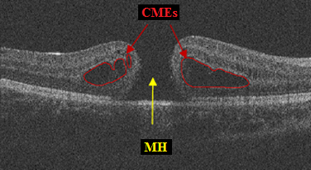ne).

There are several previous studies focused on the segmentation of CMEs. Both semiautomated and automated methods have been studied. The semiautomated methods rely on manual initialization in each B-scan to quantify the volume of CMEs. Kashani et al.¹¹ used the OCTOR software to quantify the cystoid spaces in eyes. Fernández¹² proposed a method that requires the manual initialization of the snake and the fluid regions in 2-D OCT B-scans can be detected using a deformable model. Zheng et al.¹³ developed a technique that utilized the computerized segmentation combined with the minimal expert interaction to quantify the volume of CMEs. Although the abovementioned methods can detect the volume of CMEs accurately, they are semiautomatic so that they are laborious and time-consuming. Several automated methods have also been proposed which can obtain satisfactory results. Wilkins et al.¹⁴ segmented the CMEs in 3-D OCT images by thresholding and boundary tracing. Roychowdhury et al.¹⁵ localized cysts in diabetic macular edema (DME) by iterative high-pass filtering with further analysis using solidity, mean, and maximum pixel value as decisive features. Sisternes et al.¹⁶ segmented the cysts in 3-D OCT images using lasso regularization-based regression and adaptive thresholding. Esmaeili et al.¹⁷ proposed a 3-D curvelet transform-based dictionary learning method for automatic segmentation of cysts. Girish et al.¹⁸ proposed a marker-controlled watershed transform-based method to segment cysts on 2-D OCT B-scan images. Venhuizen et al.¹⁹ proposed a multiscale convolutional neural network-based method to predict if an image voxel belongs to a cyst. Wang et al.²⁰ proposed a fuzzy level set-based method to automatically segment the intraretinal fluid and subretinal fluid in DME eyes using structural OCT and angiography OCT data. However, these methods may fail when the MH and CMEs coexist. There may be two reasons. First, most of the CMEs segmentation methods in OCT images are based on the intensity differences between CMEs and the other tissues of retina, and the intensity of MH is similar to the one of CMEs, so MH may be very likely segmented as a false positive (FP) region. Second, some of the above methods, e.g., Sisternes et al.¹⁶ use the position information about the fovea center because CMEs usually surround the fovea. When MH co-occurs, the normal shape of retina is altered and the correct position of the fovea center cannot be detected. This may be another cause of FPs. Therefore, new methods that can fully segment the CMEs in the retina with MH are urgently needed.

The automatic segmentation of the CMEs coexisting with the MH is a challenging problem. The key difficulties lie in two aspects: (1) MH is a great disturbance for CMEs segmentation, and MH cannot be easily segmented because the shapes of the MHs may be irregular and even distorted by the detached tissues, such as posterior vitreous detachment.²¹ (2) The number and size of CMEs are always uncertain, making it difficult to quantify the volume of the cysts.

In this paper, we propose an automated framework for intraretinal CME segmentation in 3-D OCT images with MH. The proposed method consists of two steps: preprocessing and CMEs segmentation. In the preprocessing, the operations including signal-to-noise (SNR)-balancing, 3-D curvature anisotropic diffusion filtering, layer segmentation and flattening, and MH and vessel silhouettes exclusion, are applied to the OCT scans. In the CMEs segmentation, first, an AdaBoost classifier with 57 features is employed for the coarse segmentation. Second, the morphological dilation and erosion operations are used to generate the foreground (CMEs) seeds and background seeds for the following graph cut-based segmentation method. Third, an automatic shape-constrained graph cut algorithm is applied for the fine segmentation. Finally, the FPs are eliminated according to the CMEs area-related information. The flowchart of the proposed method is shown in Fig. 2.

Fig. 2

The flowchart of the proposed method.

2. Materials and Methods

2.1.

Subjects and Data Collection

The collection and analysis of image data were approved by the Institutional Review Board of Joint Shantou International Eye Center (JSIEC), Shantou University and the Chinese University of Hong Kong and adhered to the tenets of the Declaration of Helsinki. Because of its retrospective nature, informed consent was not required from subjects. The medical records and OCT database of JSIEC from December 2008 to 2013 were searched and reviewed.

Totally, 19 eyes with coexistence of CMEs and MH from 18 subjects were included and underwent macular-centered ( $6 \times 6 mm$ ) SD-OCT scan (Topcon 3-D OCT-1000, $512 \times 32 \times 480 voxels$ , $11.72 \times 187.5 \times 3.50 μ m^{3}$ , $512 \times 64 \times 480 voxels$ , $11.72 \times 93.75 \times 3.50 μ m^{3}$ , or $512 \times 128 \times 480 voxels$ , $11.72 \times 46.88 \times 3.50 μ m^{3}$ ). There were 8 males and 10 females with the mean age of $45.6 \pm 19.7$ years (range: 9 to 66 years). Subjects with other eye diseases were excluded except for refractive error $< = \pm 6$ diopter. The raw, uncompressed data were exported from the OCT machine as “.fds” format for analysis.

2.2.

Ground Truth Delineation

All the CME regions in the 3-D OCT images were manually marked slice by slice by two observers independently, under the directions of an experienced ophthalmologist. The marked results marked are considered as the ground truth one (GT1) and ground truth two (GT2), respectively.

2.3.

Preprocessing

The OCT volume is first segmented into 10 layers by 11 surfaces using the multiscale 3-D graph-search approach.²²^–²⁵ To remove the image deformation caused by eye movement, the 3-D OCT volume is flattened based on the retinal pigment epithelium (surface 11).²⁶^–²⁸ The inner retina is defined as the region between surfaces 1 and 6, and the outer retina refers to the region between surfaces 7 and 11. As the CMEs are mainly located in the inner retina, the inner retina is our initial volume of interest (VOI). So the precise segmentation of surfaces 1 and 6 is necessary. As shown in Fig. 3(b), surface 6 is well detected by the 3-D graph-search-based approach except the region around the CMEs, due to the coexistence of CMEs and MH. Surface 6 is then adjusted by replacing it with the lower boundary of its convex hull.²⁹ Figure 3(c) shows the results after adjustment.

Fig. 3

Illustration of layer segmentation and adjustment. (a) One slice from the original 3-D OCT image. (b) Layer segmentation results of surface 1 (red) and surface 6 (purple) by the graph-search method. (c) Layer segmentation after surface 6 adjustment.

The OCT images acquired from different patients have different intensity profiles, which will affect the CMEs segmentation. In this paper, a SNR balancing¹⁴ is used on each B-scan to obtain uniform intensity profile. The noise level $N$ is taken as the mean intensity within a $20 \times 20$ window in the background. The signal level $S$ is taken as the mean intensity within a $20 \times 20$ window in the region between surfaces 1 and 6. The image data are SNR balanced using the equation $I_{SNR} = (I_{O} - N) / (S - N)$ , where $I_{O}$ is the original intensity value and $I_{SNR}$ is the final intensity value.

Speckle noise is the main quality-degrading factor in OCT scans. The denoising method applied to OCT images should be efficient for speckle noise suppression while maintaining edge-like features. A 3-D curvature anisotropic diffusion filter is adopted in this paper. This filter performs anisotropic diffusion using the modified curvature diffusion equation (MCDE),³⁰ which can efficiently enhance the contrast of edges. The MCDE equation is given as

Eq. (1)

f_{t} = | \nabla f | \nabla \cdot c (| \nabla f |) \frac{\nabla f}{| \nabla f |},

where

f

denotes the input image,

c

is the conductance function. The conductance modified curvature term is

\nabla \cdot \frac{\nabla f}{| \nabla f |}

. Figure 4(b) shows a B-scan image after the 3-D curvature anisotropic diffusion filtering, in which the speckle noise is effectively reduced.

Fig. 4

SNR balancing results followed by a 3-D curvature anisotropic diffusion filtering. (a) Original B-scan and (b) denoised B-scan.

2.4.

Macular Hole Detection and Vessel Silhouettes Exclusion

Because the MH and vessel silhouettes have similar intensity value to the CMEs, it is necessary to isolate the MH and vessel silhouettes before extracting the CMEs volumetric feature. This procedure can reduce the volume of data to be analyzed and reduce the FPs.

The likelihood that a point belongs to an MH footprint can be calculated from the 2-D projection image in $X - Y$ plane.³¹ Here, a 2-D projection image is generated by averaging the OCT subvolume between surfaces 1 and 6 in the $z$ -direction, as shown in Fig. 5(a). Then a footprint of MH is defined by thresholding [ $threshold value = 33$ , in range (0, 255)]. The initial result is shown in Fig. 5(b). Because the footprint of MH usually locates around the center of the 2-D projection image, the falsely detected regions nearby the border, caused by signal attenuation, are discarded. The final result of the MH footprint is shown in Fig. 5(c).

Fig. 5

MH footprint detection. (a) The 2-D projection image ( $X - Y$ plane) from surfaces 1 to 6. (b) Rough detection results by thresholding. (c) MH footprint detection result after removing FPs.

With the detected MH footprint, an improved region-growing method is applied to delineate the MH in the 3-D OCT image. First, the seeds for region growing are determined based on the following criteria:

1. belonging to the A-scans indicated by the 2-D MH footprint,
2. between surfaces 1 and 6,
3. with intensity smaller than $m_{M H} + {std}_{M H}$ , in which $m_{M H}$ and ${std}_{M H}$ are the statistical mean intensity and standard deviation of the MH region, respectively.

Second, with the detected seeds, the region-growing method becomes automatic. The neighbors of the seeds are searched and determined whether they belong to the object region according to intensity.

The CMEs segmentation results may occasionally include the low-intensity regions, such as vessel silhouettes, which are shown in Fig. 6. The arrows indicate vessel silhouettes formed by the vasculature of the retina. The green line in (b) indicates the location of the slice shown in (a) on the projection image of the retina. The vessel silhouettes should be detected and excluded before the CMEs segmentation. Here, the vessel silhouettes are effectively detected using a vessel detector.³² First, a 2-D projection image [Fig. 6(b)] is calculated by averaging the intensities of pixels in the outer retina (from surfaces 7 to 12) in the $z$ -direction, as the vessel silhouettes have excellent contrast only in the outer retina. Then the vessel silhouettes are segmented from the projection image by a KNN classifier with 31 features. Finally, if the voxels in the inner retina regions have the same $x$ , $y$ locations with the vessel silhouettes, they are excluded from the VOI.

Fig. 6

Vessel silhouettes appear as low-intensity regions which may cause FPs. (a) The arrows indicate vessel silhouettes on a B-scan image. (b) The green line indicates the location of the slice shown in (a) on the projection image.

At last, the subvolume of the retina between surfaces 1 and 6 without the MH and the vessel silhouettes is defined as our real VOI.

2.5.

AdaBoost Classifier-Based Coarse Cystoid Macular Edemas Segmentation

After preprocessing, 57 features are extracted for each voxel in the VOI, including textural and structural information of the image. Table 1 shows the list of features. Features 1 to 8 describe the local texture of the image. The first 6 features were defined in our previous research.³³ The skewness and kurtosis are used to describe the statistical distribution characteristics of the intensity values in the VOI. Features 9 to 57 describe the local image structure. In order to speed up the feature extraction phase, the training images are sampled which yielded images of $256 \times 240 \times 32 voxels$ . Then, an AdaBoost classifier is applied for the coarse segmentation of CMEs in the VOI. AdaBoost is an iterative boosting algorithm constructing a strong classifier as a linear combination of weak classifiers.³⁴^,³⁵ The algorithm takes the set of $(x_{1}, y_{1}), (x_{2}, y_{2}), \dots, (x_{n}, y_{n})$ as the input, where $x_{i} (i = 1,2, \dots, n)$ is a $m$ -dimensional feature, and $y_{i} (i = 1,2, \dots, n)$ is the corresponding label, set as 1 or 0 for cyst or noncyst voxels. In this paper, $m = 57$ .

Table 1

List of the features used in the AdaBoost classifier.

Feature number	Feature description
1	Max–min normalized intensity
2 to 3	Block mean intensity and standard deviation (block size: $3 \times 3 \times 3$ )
4 to 6	Gradient in three directions
7 to 8	Skewness and kurtosis
9 to 13	First eigenvalues of the Hessian matrix at $scales = 1$ , 3, 6, 9, 14
14 to 18	Second eigenvalues of the Hessian matrix at $scales = 1$ , 3, 6, 9, 14
19 to 23	Third eigenvalues of the Hessian matrix at $scales = 1$ , 3, 6, 9, 14
24 to 53	Gaussian filter banks of zero, first, and second orders with derivatives at $scales = 2$ , 4, 8
54 to 57	Occurrence matrix contrast, correlation, energy, and homogeneity

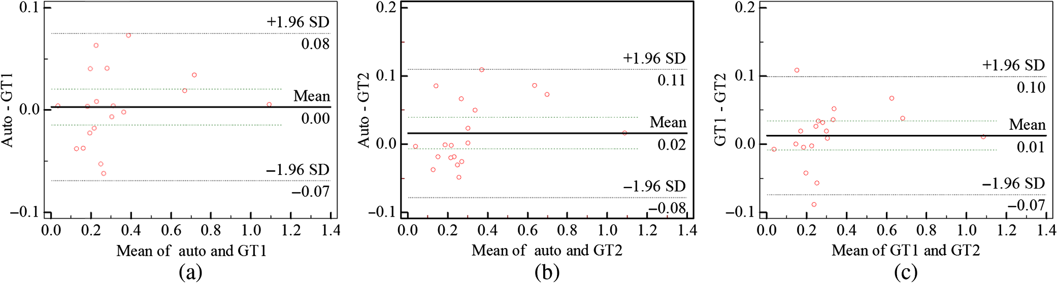
The coarsely detected CME regions are processed by the morphological dilation and erosion operations, to generate the object and background seeds for the following graph cut-based fine CMEs segmentation.

2.6.

Constrained Graph Cut-Based Fine Cystoid Macular Edemas Segmentation

The graph cut algorithm has been widely used for the image segmentation in recent years.³⁶^–⁴⁰ The energy function of traditional graph cut includes a regional term and boundary term. Obtaining seeds is an important step of the graph cut algorithm. With the given seeds generated in the coarse segmentation step, an automated shape-constrained graph cut method is applied for the final fine segmentation.⁴¹ In the graph cut algorithm, the overall problem can be formulated as an energy minimization problem.⁴² The energy function of the shape-constrained graph cut is defined as

Eq. (2)

E (l) = \sum_{p \in P} [α D_{p} (l_{p}) + β S_{p} (l_{p})] + \sum_{p \in P, q \in N_{p}} γ B_{p, q} (l_{p}, l_{q}),

where

α

,

β

,

γ

denote the weights for the data term, shape term, and boundary term, respectively. They satisfy

α + β + γ = 1

. The data term is defined as a probability of the voxel to be the object or not. The boundary term is defined on the gradient of the intensity between the adjacent voxels. They are defined as follows:

Eq. (3)

D_{p} (l_{p}) = {\begin{cases} - \ln P (I_{p} | O), & if l_{p} is object label \\ - \ln P (I_{p} | B), & if l_{p} is background label \end{cases},

Eq. (4)

B_{p, q} (l_{p}, l_{q}) = \exp [- \frac{{(I_{p} - I_{q})}^{2}}{2 σ^{2}}] \frac{1}{d (p, q)} δ (l_{p}, l_{q}),

and

Eq. (5)

δ (l_{p}, l_{q}) = {\begin{cases} 0, & if l_{p} \neq l_{q} \\ 1, & otherwise \end{cases},

where

I_{p}

is the intensity of the voxel

p

and

l_{p}

is the label assigned to the voxel

p

.

P (I_{p} | O)

and

P (I_{p} | B)

represent the probabilities that the voxel

p

belongs to CME and non-CME, respectively. They can be calculated from the histogram of the CME and non-CME voxels during the training phase.

d (p, q)

is the distance between voxel

p

and

q

.

σ

is the standard deviation of the voxel intensity.

The shape term is defined as,

Eq. (6)

S_{p} (l_{p}) = 1 - \exp [- \frac{d (p, CME)}{r}],

where

d (p, CME)

is the distance from voxel

p

to the coarse CMEs segmentation result in the AdaBoost classification.

r

is the radius of a circle that can just enclose the CMEs. The shape-constrained graph cut is implemented on the VOI and the CMEs region can be refined.

2.7.

False Positive Rejection

The CMEs FPs may be caused by the noise and the retinal region with low intensity value. The connected component detection based on morphological operations is used to reject the FPs. If the area of the detected connected region is smaller than 6 pixels, it will be discarded as an FP.

3. Results

Leave-one-out cross-validation strategy was used for training and testing the AdaBoost classifier and the parameters used in the graph cut. To objectively evaluate the CME volume segmentation results, the true positive volume fraction (TPVF), FP volume fraction (FPVF), accuracy rate (ACC), and dice similarity coefficient (DSC) are used in the experiment.⁴³^,⁴⁴ TPVF indicates the rate of correctly detected volume compared with the reference standard. FPVF denotes the fraction of incorrectly detected volume in the true negative volume. ACC indicates the detection ACC. DSC is used for comparing the similarity between the automated segmentation results and the ground truth. The definitions are defined as follows:

Eq. (7)

TPVF = \frac{| V_{T P} |}{| V_{G T} |},

Eq. (8)

FPVF = \frac{| V_{F P} |}{| V | - | V_{G T} |},

Eq. (9)

ACC = \frac{| V_{T P} | + | V_{T N} |}{| V |},

Eq. (10)

DSC = 2 \times \frac{| V_{T P} |}{| V_{T P} | + | V_{F P} | + | V_{G T} |},

where

| \cdot |

denotes volume,

V_{T P}

denotes the true positive set,

V_{F P}

denotes the FP set,

V_{T N}

denotes the true negative set, and

V_{F N}

denotes the false negative set.

V_{G T}

denotes the ground truth, and

V

denotes the VOI.

As shown in Table 2, the mean of TPVF, FPVF, ACC, and DSC for the proposed method was 81.0%, 0.80%, 99.7%, and 80.9%, respectively. The proposed method was compared with the coarse CMEs segmentation based only on the AdaBoost algorithm, the 2-D thresholding segmentation method proposed in Ref. 14, and the lasso regularization-based regression method proposed in Ref. 16. Compared to the results by the AdaBoost algorithm, the DSC of the proposed method increased slightly (with a $p$ -value of 0.061 in the paired $t$ -test) and the corresponding ACC showed a significant improvement (with a $p$ -value $< 0.0001$ ). The results of the proposed 3-D method showed a more significant improvement compared to the results of the 2-D thresholding segmentation proposed in Ref. 14. Though the average TPVF of the regression method proposed in Ref. 16 is higher than the proposed method, its FPVF, ACC, and DSC are much poorer than the ones of the proposed method, which is caused by large FP regions.

Table 2

Mean±standard deviation comparison of the CMEs segmentation results.

	TPVF (%)	FPVF (%)	ACC (%)	DSC (%)
Ref. 14	$72.5 \pm 17.6$	$8.3 \pm 5.6$	$82.5 \pm 3.2$	$71.2 \pm 6.8$
Ref. 16	$90.5 \pm 12.3$	$8.3 \pm 5.9$	$91.9 \pm 5.0$	$53.5 \pm 11.0$
AdaBoost-only	$79.5 \pm 8.7$	$0.80 \pm 0.42$	$98.1 \pm 0.6$	$79.1 \pm 7.2$
Proposed method	$81.0 \pm 7.8$	$0.80 \pm 0.63$	$99.7 \pm 0.1$	$80.9 \pm 5.7$

Figure 7 shows five examples of CMEs segmentation results. The first column shows the original image, the second column shows the coarse segmentation results of the AdaBoost classifier, the third column shows the final fine segmentation results, the fourth column shows the segmentation results by 2-D thresholding segmentation method proposed in Ref. 14, the fifth column shows the segmentation results by lasso regularization-based regression method proposed in Ref. 16, and the last column shows the GT1. Note the improvements between columns 2 and 3. There are FPs caused by the presence of MH in columns 3 and 4.

Fig. 7

Experimental results for five examples of CMEs segmentation. The first column shows the original image, the second column shows the segmentation results of AdaBoost classifier, the third column shows the final fine segmentation results, the fourth column shows the segmentation results by 2-D thresholding segmentation method proposed in Ref. 14, the fifth column shows the segmentation results by lasso regularization-based regression method proposed in Ref. 16, and the last column shows the GT1.

Figure 8 shows the linear regression analysis results for the GT1 versus the GT2. The correlation $R^{2}$ between the proposed method and GT1, GT2, and the average of GT1 and GT2 were 0.9794, 0.9668, and 0.9812, respectively. The correlation coefficient between GT1 and GT2 was 0.9677, which indicated the two ground truths are very consistent.

Fig. 8

Statistical correlation analysis between the automated method, GT1 and GT2. (a) The linear regression analysis results between GT1 and the automatic method. (b) The linear regression analysis results between GT2 and the automatic method. (c) The linear regression analysis results between the automatic method and the average of GT1 and GT2. (d) The linear regression analysis results between GT1 and GT2.

Figure 9 shows the CMEs volume of 19 subjects by three methods. Bland and Altman plots were used to evaluate the agreement between two different methods. The Bland–Altman plots for the proposed method (auto) versus the GT1 and the GT2 are shown in Fig. 10. The points were mostly located in the 95% limits of agreement ( $\pm 1.96$ standard deviation of the difference), which indicated good agreement between the proposed method and GT1 and GT2.

Fig. 9

Bar plot for CMEs volume comparison.

Fig. 10

Bland–Altman plot of CME volume. (a) Bland–Altman plot for auto versus GT1. (b) Bland–Altman plot for auto versus GT2. (c) Bland–Altman plot for GT1 versus GT2.

4. Discussion and Conclusions

Automated segmentation of CMEs in 3-D OCT images is a challenging task due to the variation of CMEs’ shape and size and the textural similarity between the foreground and background. The experiment results showed the good performance of the proposed method. The FPVF of the proposed method was low, which may be due to several facts: (1) compared with the VOI region between surfaces 1 and 6, the volume of the CMEs is very small; (2) the size for FP exclusion in the postprocessing is very effective. The CMEs can be effectively segmented by the proposed method. With coexistence of MH, both the 2-D thresholding method proposed in Ref. 14 and the lasso regularization-based regression method proposed in Ref. 16 fail to exclude the MH effectively, because the intensity value is similar between MH and CMEs and neither of these two methods uses the spatial and shape information about the MH.

Our contributions are summarized as follows:

• This is a method for the automated 3-D CMEs volume segmentation in the retina with coexistence of MH.
• The proposed method can effectively detect CMEs with unpredictable locations and ambiguous boundaries (as shown in Fig. 11).
• An improved efficient region-growing method is proposed to delineate the MH in 3-D OCT image.
• The seeds used in the shape-constrained graph cut algorithm are generated automatically and the proposed method is a fully automated framework.

Fig. 11

Segmentation results for CMEs with unpredictable locations and ambiguous boundaries. The first column shows the original image, the second column shows the segmentation results of the proposed method, and the third column shows the GT1.

However, there are still some limitations in our method. (1) The proposed method can accurately detect a big cyst, but it is not sensitive to very small cysts. This will be improved in the near future. (2) The final CMEs detection results largely rely on the preprocessed results. If the MH exclusion result is incorrect, the final segmentation results may include falsely detected regions in MH. A better algorithm for MH detection is needed. (3) A larger dataset will be explored in the near future for further validation of the proposed method.

In conclusion, an effective approach is proposed to segment the CMEs in the 3-D OCT images with coexistence of MH. This may provide a clinically useful tool to help ophthalmologists with disease diagnosis.

Disclosures

Li Zhang has a financial interest in Oracle Inc., which, however, did not support this work. No conflicts of interest, financial or otherwise, are declared by the other authors.

Acknowledgments

This study was supported by the National Basic Research Program of China (973), the Young Scientist Program Foundation of China (2014CB748600), the National Nature Science Foundation of China (81401472) and in part by the National Nature Science Foundation of China for Excellent Young Scholars (61622114), the National Nature Science Foundation of China (61401294, 61401293, and 81371629), the Natural Science Foundation of Jiangsu Province (BK20140052), the International Cooperation Project of Ministry of Science and Technology (2016YFE010770), and the Research Grant from the Joint Shantou International Eye Center (2012–2018).

References

1.

M. D. Abràmoff, M. K. Garvin and M. Sonka, “Retinal imaging and image analysis,” IEEE Rev. Biomed. Eng., 3 169 –208 (2010). http://dx.doi.org/10.1109/RBME.2010.2084567 Google Scholar

2.

C. Cukras et al., “Optical coherence tomography-based decision making in exudative age-related macular degeneration: comparison of time vs spectral-domain devices,” Eye, 24 (5), 775 –783 (2010). http://dx.doi.org/10.1038/eye.2009.211 12ZYAS 0950-222X Google Scholar

3.

D. Huang et al., “Optical coherence tomography,” Science, 254 (5035), 1178 –1181 (1991). http://dx.doi.org/10.1126/science.1957169 SCIEAS 0036-8075 Google Scholar

4.

E. A. Swanson et al., “In vivo retinal imaging by optical coherence tomography,” Opt. Lett., 18 (21), 1864 –1866 (1993). http://dx.doi.org/10.1364/OL.18.001864 OPLEDP 0146-9592 Google Scholar

5.

Y. Liu et al., “Automated macular pathology diagnosis in retinal OCT images using multi-scale spatial pyramid and local binary patterns in texture and shape encoding,” Med. Image Anal., 15 (5), 748 –759 (2011). http://dx.doi.org/10.1016/j.media.2011.06.005 Google Scholar

6.

H. Faghihi et al., “Spontaneous closure of traumatic macular holes,” Can. J. Ophthalmol., 49 (4), 395 –398 (2014). http://dx.doi.org/10.1016/j.jcjo.2014.04.017 CAJOBA 0008-4182 Google Scholar

7.

W. E. Smiddy and H. W. Flynn, “Pathogenesis of macular holes and therapeutic implications,” Am. J. Ophthalmol., 137 (3), 525 –537 (2004). http://dx.doi.org/10.1016/j.ajo.2003.12.011 AJOPAA 0002-9394 Google Scholar

8.

A. Luckie and W. Heriot, “Macular holes. Pathogenesis, natural history and surgical outcomes,” J. Ophthalmol., 23 (2), 93 –100 (1995). http://dx.doi.org/10.1111/j.1442-9071.1995.tb00136.x Google Scholar

9.

T. G. Rotsos and M. M. Moschos, “Cystoid macular edema,” Clin. Ophthalmol., 2 (4), 919 –930 (2008). http://dx.doi.org/10.2147/OPTH Google Scholar

10.

L. Pelosini et al., “Optical coherence tomography may be used to predict visual acuity in patients with macular edema,” Invest. Ophthalmol. Visual Sci., 52 (5), 2741 –2748 (2011). http://dx.doi.org/10.1167/iovs.09-4493 IOVSDA 0146-0404 Google Scholar

11.

A. H. Kashani et al., “Quantitative subanalysis of cystoid spaces and outer nuclear layer using optical coherence tomography in age-related macular degeneration,” Invest. Ophthalmol. Visual Sci., 50 (7), 3366 –3373 (2009). http://dx.doi.org/10.1167/iovs.08-2691 IOVSDA 0146-0404 Google Scholar

12.

D. C. Fernández, “Delineating fluid-filled region boundaries in optical coherence tomography images of the retina,” IEEE Trans. Med. Imaging, 24 (8), 929 –945 (2005). http://dx.doi.org/10.1109/TMI.2005.848655 ITMID4 0278-0062 Google Scholar

13.

Y. Zheng et al., “Computerized assessment of intraretinal and subretinal fluid regions in spectral-domain optical coherence,” Am. J. Ophthalmol., 155 (2), 277 –286 (2013). http://dx.doi.org/10.1016/j.ajo.2012.07.030 AJOPAA 0002-9394 Google Scholar

14.

G. R. Wilkins, O. M. Houghton and A. L. Oldenburg, “Automated segmentation of intraretinal cystoid fluid in optical coherence tomography,” IEEE Trans. Biomed. Eng., 59 (4), 1109 –1114 (2012). http://dx.doi.org/10.1109/TBME.2012.2184759 IEBEAX 0018-9294 Google Scholar

15.

S. Roychowdhury et al., “Automated localization of cysts in diabetic macular edema using optical coherence tomography images,” in 35th Annual Int. Conf. of the IEEE Engineering in Medicine and Biology Society (EMBC 2013), 1426 –1429 (2013). http://dx.doi.org/10.1109/EMBC.2013.6609778 Google Scholar

16.

L. D. Sisternes et al., “A machine learning approach for device-independent automated segmentation of retinal cysts in spectral domain optical coherence tomography images,” in Proc. MICCAI 2015 OPTIMA Challenge, (2015). Google Scholar

17.

M. Esmaeili et al., “Three-dimensional segmentation of retinal cysts from spectral-domain optical coherence tomography images by the use of three-dimensional curvelet based K-SVD,” J. Med. Signals Sens., 6 (3), 166 –171 (2016). Google Scholar

18.

G. N. Girish, A. R. Kothari and J. Rajan, “Automated segmentation of intra-retinal cysts from optical coherence tomography scans using marker controlled watershed transform,” in IEEE 38th Annual Int. Conf. of the Engineering in Medicine and Biology Society (EMBC 2016), 1292 –1295 (2016). http://dx.doi.org/10.1109/EMBC.2016.7590943 Google Scholar

19.

F. Venhuizen et al., “Fully automated segmentation of intraretinal cysts in 3D optical coherence tomography,” in ARVO Annual Meeting Abstract, 5949 (2016). Google Scholar

20.

J. Wang et al., “Automated volumetric segmentation of retinal fluid on optical coherence tomography,” Biomed. Opt. Express, 7 (4), 1577 –1589 (2016). http://dx.doi.org/10.1364/BOE.7.001577 BOEICL 2156-7085 Google Scholar

21.

U. C. Christensen, “Value of internal limiting membrane peeling in surgery for idiopathic macular hole and the correlation between function and retinal morphology,” Acta Ophthalmol., 87 1 –23 (2009). http://dx.doi.org/10.1111/j.1755-3768.2009.01777.x ACOPAT 0001-639X Google Scholar

22.

K. Li et al., “Optimal surface segmentation in volumetric images-a graph-theoretic approach,” IEEE Trans. Pattern Anal. Mach. Intell., 28 (1), 119 –134 (2006). http://dx.doi.org/10.1109/TPAMI.2006.19 ITPIDJ 0162-8828 Google Scholar

23.

X. J. Chen et al., “3D segmentation of fluid-associated abnormalities in retinal OCT: probability constrained graph-search–graph-cut,” IEEE Trans. Med. Imaging, 31 (8), 1521 –1531 (2012). http://dx.doi.org/10.1109/TMI.2012.2191302 ITMID4 0278-0062 Google Scholar

24.

F. Shi et al., “Automated 3-D retinal layer segmentation of macular optical coherence tomography images with serous pigment epithelial detachments,” IEEE Trans. Med. Imaging, 34 (2), 441 –452 (2015). http://dx.doi.org/10.1109/TMI.2014.2359980 ITMID4 0278-0062 Google Scholar

25.

F. Shi et al., “Automated choroid segmentation in three-dimensional 1-μm wide-view OCT images with gradient and regional costs,” J. Biomed. Opt., 21 (12), 126017 (2016). http://dx.doi.org/10.1117/1.JBO.21.12.126017 JBOPFO 1083-3668 Google Scholar

26.

X. J. Chen et al., “Quantification of external limiting membrane disruption caused by diabetic macular edema from SD-OCT,” Invest. Ophthalmol. Visual Sci., 53 (13), 8042 –8048 (2012). http://dx.doi.org/10.1167/iovs.12-10083 IOVSDA 0146-0404 Google Scholar

27.

M. K. Garvin et al., “Automated 3-D intrarential layer segmentation of macular spectral-domain optical coherence tomography images,” IEEE Trans. Med. Imaging, 28 (9), 1436 –1447 (2009). http://dx.doi.org/10.1109/TMI.2009.2016958 ITMID4 0278-0062 Google Scholar

28.

K. Lee et al., “Segmentation of the optic disc in 3-D OCT scans of the optic nerve head,” IEEE Trans. Med. Imaging, 29 (1), 159 –168 (2010). http://dx.doi.org/10.1109/TMI.2009.2031324 ITMID4 0278-0062 Google Scholar

29.

R. C. Gonzalez, R. E. Woods and S. L. Eddins, Digital Image Processing Using MATLAB, Pearson Prentice-Hall, New Jersey (2004). Google Scholar

30.

R. Whitaker and X. Xue, “Variable-conductance, level-set curvature for image denoising,” in Proc. of the Int. Conf. on Image Processing, 142 –145 (2010). http://dx.doi.org/10.1109/ICIP.2001.958071 Google Scholar

31.

G. Quellec et al., “Three-dimensional analysis of retinal layer texture: identification of fluid-filled regions in SD-OCT of the macula,” IEEE Trans. Med. Imaging, 29 (6), 1321 –1330 (2010). http://dx.doi.org/10.1109/TMI.2010.2047023 ITMID4 0278-0062 Google Scholar

32.

M. Niemeijer et al., “Vessel segmentation in 3D spectral OCT scans of the retina,” Proc. SPIE, 6914 69141R (2008). http://dx.doi.org/10.1117/12.772680 PSISDG 0277-786X Google Scholar

33.

L. Y. Wang et al., “Support vector machine based IS/OS disruption detection from SD-OCT images,” Proc. SPIE, 9034 90341U (2014). http://dx.doi.org/10.1117/12.2043439 PSISDG 0277-786X Google Scholar

34.

C. A. Lupascu, D. Tegolo and E. Trucco, “FABC: retinal vessel segmentation using AdaBoost,” IEEE Trans. Inf. Technol. Biomed., 14 (5), 1267 –1274 (2010). http://dx.doi.org/10.1109/TITB.2010.2052282 Google Scholar

35.

X. Li, L. Wang and E. Sung, “AdaBoost with SVM-based component classifiers,” Eng. Appl. Artif. Intell., 21 (5), 785 –795 (2008). http://dx.doi.org/10.1016/j.engappai.2007.07.001 EAAIE6 0952-1976 Google Scholar

36.

X. J. Chen and U. Bağci, “3D automatic anatomy segmentation based on iterative graph-cut-ASM,” Med. Phys., 38 (8), 4610 –4622 (2011). http://dx.doi.org/10.1118/1.3602070 MPHYA6 0094-2405 Google Scholar

37.

Y. Boykov and G. Funka-Lea, “Graph cuts and efficient N–D image segmentation,” Int. J. Comput. Vision, 70 (2), 109 –131 (2006). http://dx.doi.org/10.1007/s11263-006-7934-5 IJCVEQ 0920-5691 Google Scholar

38.

X. J. Chen et al., “Medical image segmentation by combining graph cut and oriented active appearance models,” IEEE Trans. Image Process., 21 (4), 2035 –2046 (2012). http://dx.doi.org/10.1109/TIP.2012.2186306 IIPRE4 1057-7149 Google Scholar

39.

Y. Y. Boykov and M. P. Jolly, “Interactive graph cuts for optimal boundary & region segmentation of objects in N-D Images,” in Proc. of the Eighth IEEE Int. Conf. on Computer Vision (ICCV 2001), 105 –112 (2001). http://dx.doi.org/10.1109/ICCV.2001.937505 Google Scholar

40.

X. J. Chen et al., “GC-ASM: synergistic integration of graph-cut and active shape model strategies for medical image segmentation,” Comput. Vision Image Understanding, 117 (5), 513 –524 (2013). http://dx.doi.org/10.1016/j.cviu.2012.12.001 CVIUF4 1077-3142 Google Scholar

41.

X. J. Chen et al., “A framework of whole heart extracellular volume fraction estimation for low dose cardiac CT images,” IEEE Trans. Inf. Technol. Biomed., 16 (5), 842 –851 (2012). http://dx.doi.org/10.1109/TITB.2012.2204405 Google Scholar

42.

Y. Boykov and V. Kolmogorov, “An experimental comparison of min-cut/max-flow algorithms for energy minimization in vision,” IEEE Trans. Pattern Anal. Mach. Intell., 26 (9), 1124 –1137 (2004). http://dx.doi.org/10.1109/TPAMI.2004.60 ITPIDJ 0162-8828 Google Scholar

43.

J. K. Udupa et al., “A framework for evaluating image segmentation algorithms,” Comput. Med. Imaging Graphics, 30 (2), 75 –87 (2006). http://dx.doi.org/10.1016/j.compmedimag.2005.12.001 CMIGEY 0895-6111 Google Scholar

44.

W. Ju et al., “Random walk and graph cut for co-segmentation of lung tumor on PET-CT images,” IEEE Trans. Image Process., 24 (12), 5854 –5867 (2015). http://dx.doi.org/10.1109/TIP.2015.2488902 IIPRE4 1057-7149 Google Scholar

Biography

Weifang Zhu is an associate professor at Soochow University, Suzhou, China. She received her PhD in electrical engineering from Soochow University, China, in 2013. She has coauthored over 15 papers in internationally recognized journals and conferences. Her current research is focused on medical image processing and analysis.

Xinjian Chen is a distinguished professor at Soochow University, Suzhou, China. He received a PhD from the Chinese Academy of Sciences in 2006. He conducted postdoctoral research in the University of Pennsylvania, National Institute of Health, and University of Iowa, USA from 2008 to 2012. He has published over 80 top international journals and conference papers. He has also been awarded six patents.

Biographies for the other authors are not available.

Citation Download Citation

Weifang Zhu, Li Zhang, Fei Shi, Dehui Xiang, Lirong Wang, Jingyun Guo, Xiaoling Yang, Haoyu Chen, and Xinjian Chen "Automated framework for intraretinal cystoid macular edema segmentation in three-dimensional optical coherence tomography images with macular hole," Journal of Biomedical Optics 22(7), 076014 (21 July 2017). https://doi.org/10.1117/1.JBO.22.7.076014

Received: 11 March 2017; Accepted: 5 July 2017; Published: 21 July 2017

Access the abstract

JOURNAL ARTICLE
9 PAGES

DOWNLOAD PAPER SAVE TO MY LIBRARY

GET CITATION

CITATIONS

Cited by 10 scholarly publications.

Explore citations on Lens.org

RIGHTS & PERMISSIONS

Get copyright permission Get copyright permission on Copyright Marketplace

Subscribe to Digital Library

Receive Erratum Email Alert

1.

Introduction

Fig. 1

Fig. 2

2.

Materials and Methods

2.1.

Subjects and Data Collection

2.2.

Ground Truth Delineation

2.3.

Preprocessing

Fig. 3

Eq. (1)

Fig. 4

2.4.

Macular Hole Detection and Vessel Silhouettes Exclusion

Fig. 5

Fig. 6

2.5.

AdaBoost Classifier-Based Coarse Cystoid Macular Edemas Segmentation

Table 1

2.6.

Constrained Graph Cut-Based Fine Cystoid Macular Edemas Segmentation

Eq. (2)

Eq. (3)

Eq. (4)

Eq. (5)

Eq. (6)

2.7.

False Positive Rejection

3.

Results

Eq. (7)

Eq. (8)

Eq. (9)

Eq. (10)

Table 2

Fig. 7

Fig. 8

Fig. 9

Fig. 10

4.

Discussion and Conclusions

Fig. 11

Disclosures

Acknowledgments

References

Biography

Keywords/Phrases

Search In:

Publication Years