1.

Introduction

Blood cells have different functionalities in the human body and tissue. Red blood cells (RBCs), or erythrocytes, are the most abundant among blood cells. An erythrocyte is a discoid cell with a thick rim and thin sunken center. The main functions of erythrocytes are to absorb oxygen from the lungs, release it into tissues during circulation, and transport carbon dioxide from the tissues to the lungs. The biconcave shape of erythrocytes (doughnut-like) allows them to squeeze through capillaries that are smaller than an RBC. However, different blood abnormalities at different stages alter the original bioconcave shape of erythrocytes into different morphologies.^1–4 During blood storage in blood banks, the shape of erythrocytes changes from biconcave to flat-disk, and then to sphero-echinocyte when the storage time exceeds a few weeks. It has been proven that the transfusion of damaged RBCs can cause severe problems to body tissue and, in some cases, may lead to death.^5–9

A typical human erythrocyte RBC has a diameter of $\sim 6.4$ to $7.76\mu \mathrm{m}$¹⁰ and thickness of 2 to $3\mu \mathrm{m}$ at its thickest point.¹¹ The surface area of adult mature RBCs is $140\mu {\mathrm{m}}^2$. Under some circumstances, a mature RBC undergoes deformation into different shapes, such as echinocytes, stomatocytes, spherocytes, elliptocytes, acanthocytes, burr cells, and schizocytes among others.¹² There are cases in which different types of RBCs may exhibit similar characteristics, such as mean corpuscular volume (MCV), with tiny differences in surface area and, in some cases, constant surface area and similar shapes, which make them difficult to distinguish easily. Therefore, RBC clustering suffers from common characteristics among different kinds of RBCs. Thus, different RBCs may sometimes be categorized in the same group and result in a significant misclassification. In a conventional RBC investigation, a hematologist manually counts and classifies the cells with assistance from a microscope; this is a procedure that is tiresome, time-consuming, and susceptible to error. More specifically, the accuracy of the counting and diagnosis is affected by subjective circumstances, such as experience and fatigue, due to human exhaustion.^13–16 Many efforts have been made in RBC studies to detect abnormalities in samples before transfusion to the patient to prevent future disorders caused by the malfunction of RBCs.^17–19

According to the above discussion, we believe the utilization of clustering techniques can provide us with reasonable results. Therefore, because of the irregularly shaped groups of RBC types distributed in feature space, the density-based clustering method can be effective in this case and for overlapped RBC data. Fuzzy clustering methods are efficient unsupervised methods that can be applied in this field for regularly shaped data points.^20,21

The idea of data clustering is based on the concept that the human brain processes information as patterns rather than numerical entities. Clustering is a process that groups data observations that are similar to each other, whereas data observations of different clusters are not similar. In supervised classification methods, the data need to be labeled before applying the classification method. As RBC data from the initial phase image are unlabeled, the unsupervised method needs to be used to label and cluster them automatically. In the unsupervised method, the goal is to intrinsically group unlabeled data without predefined data groups.^20–23

In conventional two-dimensional (2-D) microscopic imaging techniques, it is difficult to detect the three-dimensional (3-D) shape of erythrocytes; thus, the overall performance is not acceptable. However, digital holographic microscopy (DHM) is capable of imaging semitransparent or transparent biological cells and provides quantitative detailed information about the cell structure and its contents at a single-RBC level. In addition, it is a noninvasive and label-free method. Therefore, samples can remain untouched for further investigations. The quantitative phase image (QPI) obtained by DHM enables us to measure the 3-D properties of RBCs, which include the volume, surface area, projected surface area (PSA), and dry mass of the biological cell.^10,11,24,25

In this study, we apply several clustering methods to cluster the different shapes of RBCs. Several RBC samples with three major morphologies, biconcave, stomatocyte, and sphero-echinocyte, are visualized by the DHM technique and are combined together. RBCs are obtained from the reconstructed phase image from the DHM technique using the watershed segmentation algorithm.^24,25 After feature extraction, similar to our previous work,¹¹ we select some good features that can efficiently discriminate between the RBC types and evaluate the clustering power of the selected features against 2-D features only. To decrease the dimensions of the features dataset, principal component analysis (PCA) is applied to the extracted features, and only three PCAs are retained. Our experimental results reveal that three PCAs can represent 90% of the entire variance. This can help us reduce the problem, enhance the clustering speed, and make the solution more efficient. In addition, the PCA technique is useful for visualizing better the 2-D and 3-D space. Eventually, several clustering methods, including density-based spatial clustering applications with noise (DBSCAN), $k$-medoids, and $k$-means clustering are applied to the dimension-reduced 2-D and 3-D features, and the clustering performance is evaluated against the 2-D features. Our experimental results show that the combination (2-D and 3-D) of features can obtain high-accuracy clustering results against 2-D features in the automated clustering of RBCs with regular shapes.

The rest of this paper is organized as follows. Section 2 is dedicated to explaining the schematic of the off-axis DHM and RBC preparation process. The image segmentation technique used in this experiment for extracting RBC samples from QPIs is briefly discussed in Sec. 3. The feature extraction process in this experiment is described in Sec. 4. DBSCAN is discussed in detail in Sec. 5. The $k$-medoids and $k$-means clustering methods are discussed in depth in Secs. 6 and 7, respectively. The experimental results and discussion on the accuracy ratio of the combination of features against the 2-D features are explained in Sec. 8. Finally, we evaluate clustering results using silhouette index (SI) in Sec. 9. We conclude the paper in Sec. 10.

2.

Off-Axis Digital Holographic Microscopy and Red Blood Cell Preparation

2.1.

Off-Axis Digital Holographic Microscopy

The off-axis DHM system uses a laser diode source of wavelength $\lambda =682\mathrm{nm}$. The laser beam is divided into two waves, the object wave and reference wave. The object wave passes through the RBC sample and gets diffracted and magnified by a microscope objective (magnification: $40\times$ and numerical aperture: 0.75); then, it interferes with the reference wave in the off-axis geometry. The interference pattern between the object and reference waves is recorded via a charge-coupled device. The QPI of the RBCs is reconstructed from the recorded interference pattern using a specific numerical algorithm.²⁶ A schematic of the off-axis DHM system is shown in Fig. 1.

Fig. 1

Schematic representation of an off-axis DHM setup.

3.

Quantitative Phase Image Segmentation of Red Blood Cells

Once we obtain an RBC QPI by the off-axis DHM system, several image-processing algorithms are applied to extract the RBCs from the reconstructed RBC QPI. The first step is to detect the correct RBC samples from the others to be extracted. Next, we remove the noise and background from the RBC QPI by applying the marker-controlled watershed segmentation algorithm to obtain segmented RBC images.^24,25 Each RBC sample is detected and extracted for analysis, and more than 14 different characteristics of every RBC sample are automatically measured.¹¹ We further explain the features we used in this paper.

Figure 2 shows the segmentation results for the automatic extraction of RBC samples from the RBC QPI obtained by the DHM system. As we mentioned, the samples we used in this study were extracted from the three main morphologies. The first sample contains the normal RBCs with a biconcave morphology [Fig. 3(a)]. The second sample contains RBCs that are suffering from the sphero-echinocyte process (other morphologies, such as biconcave, can also be found). They were stored for 57 days and then imaged by DHM. The last sample contains cells that are mostly of the stomatocyte morphology. In total, 275 single RBCs were extracted for the feature extraction section.

Fig. 2

Segmentation step: (a) original QPI obtained by off-axis DHM, (b) corresponding segmented RBC image using the marker-controlled watershed algorithm, and (c) binary-segmented RBC image (white bar indicates $10\mu \mathrm{m}$).

Fig. 3

(a) Biconcave sample, (b) RBCs suffering from sphero-echinocytes, and (c) stomatocyte sample.

4.

Feature Extraction and Selection

In this experiment, we extract over 14 2-D and 3-D features related to the RBC profile. We select the best combination of 2-D and 3-D features that can efficiently distinguish between different RBC types and another six 2-D features to compare the clustering method performance.¹¹ The first selected 3-D feature to be used in this experiment is the average cell thickness (ACT), which can be calculated by the following equation:

The fourth feature is the sphericity coefficient, which can be obtained using the following equation:

Table 1

Descriptions and feature type divisions of selected 2-D and 3-D features (best selected feature set).

In our experiment, we evaluated the clustering power of the 2-D features against the best 2-D and 3-D features. We believe that to obtain the best clustering results, we must select the major 2-D and 3-D features. The selected 2-D RBC features and their descriptions are listed in Table 2.

Table 2

Description and feature type divisions of selected 2-D RBC features.

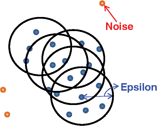
5.

Density-Based Spatial Clustering Applications with Noise

DBSCAN is a clustering method proposed by Ester et al. in 1996, which can identify clusters in large spatial data using the density of data elements. If we consider a point of data as some point distributed in space, the method groups the data points that are in close proximity to each other.²⁷ For a set of samples distributed in feature space to be clustered, DBSCAN has two main parameters, MinPts (number of $p$ points) and $ϵ$, where $p$ is the number of data points and $ϵ$ (epsilon) is the maximum radius of neighboring $p$ points. It is a nonparametric approach and considers one point as a core point if at least a minimum number of $p$ points is within a distance $ϵ$ of the core point neighborhood. In every step, the core point is changed, and the number of points reachable from the core point with the distance $ϵ$ is checked again; the core point is changed until all reachable points are met, and the unreachable points are marked as noise points.²⁸

Figure 4 shows a schematic representation of the density-based clustering method. The red points are considered as noise points. This implies that the noise data points are far from the other data points. In the DBSCAN clustering method, we need not define the number of clusters, such as in the traditional method. When a cluster is surrounded by another cluster, DBSCAN can cluster the inner and outer clusters effectively. DBSCAN selects two values as input parameters, which can effectively be adjusted according to the density of data points. This parameter can be set by an expert and also be based on data observations.²⁸

Fig. 4

Schematic representation of density-based clustering method. Epsilon and noise points are marked.

6.

$k$-Medoids Clustering Method

The $k$-medoids clustering method is a combination of two main algorithms of $k$-means and medoid shift. Both $k$-medoids and $k$-means group similar data and separate them from the other clusters.²⁹ The $k$-means clustering method is based on the minimization of the total square error, whereas $k$-medoids attempts to minimize the sum of differences between different samples in the same cluster with the medoid point, which is the center point of every cluster. $k$-medoids considers one data point as the center of a cluster. It is more powerful than the $k$-means algorithm because it is not sensitive to outliers. $k$-means is easily influenced by high-value data points in the dataset because it considers the mean of all data points, whereas $k$-medoids considers centered data points, which are more reliable.³⁰ When we have an infinite dataset, the $k$-medoids clustering method considers a data point that exhibits a minimum average dissimilarity to all the other data points. The steps of the $k$-medoids clustering algorithm are as follows:

The cost function is as follows:

7.

$k$-Means Clustering Method

The $k$-means clustering method is a popular method for clustering data observations into $k$ clusters by assigning data observations to each cluster with close distance to the mean value of all similar observations in the same cluster. This process causes the data space to be partitioned according to the mean value of similar data observations.³¹ If we consider data observations as $D=\{X_1,X_2,\dots .,X_n\}$ and the number of different clusters as $k$, the $k$-means algorithm attempts to find a $k$ centroid point $C=\{C_1,\dots ..,C_n\}$ to minimize the distance between the data and centroid point.³² The main idea of $k$-means clustering is to find the best centroid point for each cluster based on the mean value of all data observations in that cluster. During several iterations, $k$-means attempts to find the best centroid point for each cluster with the closest distance to all observations of $k$ clusters by updating the centroid point. In every iteration, the centroid point will be changed until there are no new points to change. The steps to find the best centroid point in the $k$-means clustering method are as follows:

The summation of distances can be calculated by the squared Euclidean distance error function using the following equation:³³

8.

Experimental Results and Discussion

After feature extraction, since our analysis is in 2-D and 3-D feature space, we applied PCA to reduce the data dimension into 2-D and 3-D feature space and to find a more meaningful basis or coordination of our data instead of original features. Whereas DBSCAN measures the distance of each data sample with neighboring samples using circle radius,²⁸ we used two PCA to be applied to DBSCAN method but for other method, we used three PCA since we analyze results in 3-D feature space as shown in Figs 5 and 10. Figure 5(a) presents the data distribution of the best features according to the first and second PCs. We believe that by varying the number of clusters, we should expect to observe similar morphologies categorized in the same cluster. We evaluated two and three clusters in this study. By utilizing the SI (in $k$-means clustering), the internal evaluation revealed that increasing the number of clusters decreases the accuracy of the clustering technique (data not shown). Another reason for choosing two and three clusters is that the samples are extracted from three different morphologies. Figure 5(b) shows the original data distribution based on six 2-D features.

Fig. 5

Original data distribution based on the first and second principal components (PCA1 and PCA2) of RBC types of the (a) best features and (b) 2-D features.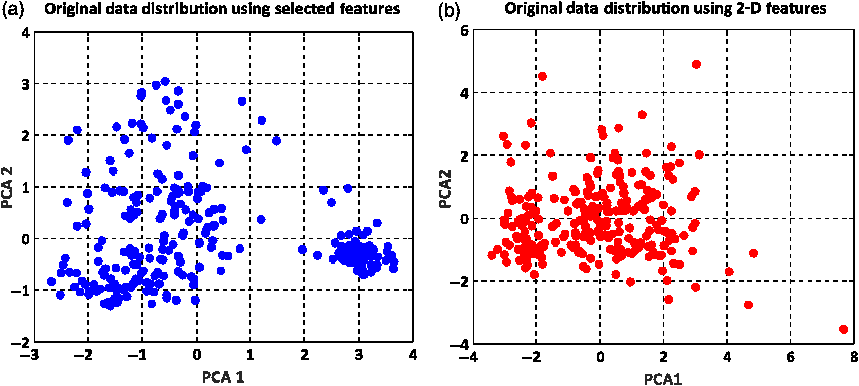

8.1.

Density-Based Spatial Clustering Applications with Noise Clustering Results

As we mentioned before, the density-based clustering approach clusters data based on the density of data observations. Therefore, this method is not based on the shape of data observations, and the number of clusters in a dataset is not predefined. Because of the density of RBC samples distributed in feature space, as shown in Fig. 5, we first applied the DBSCAN clustering algorithm and repeated the clustering experiment while varying the MinPts and epsilon parameters to find the most efficient clustering result. The MinPts parameter denotes the minimum number of data points that can be covered by the radius of a circle, which is known as the epsilon value. Concerning the selection of DBSCAN parameters, there is no special role for MinPts and epsilon parameters. They depend on density and distance of data points around the core point. A low MinPts causes more clusters to build from noise and generates more outliers, and for the epsilon parameter, it is normally considered a number between zero and one on the dataset. Hence, both parameters should not be too small or too large.

DBSCAN considers samples that are far from the other samples as noise or unknown data. This implies that these samples are considered different from the known samples. Therefore, we changed the values of MinPts and epsilon to obtain the best value for these parameters and obtain the best clustering result. In the case of clustering RBCs using DBSCAN based on the 2-D features, according to the data distribution presented in Fig. 5(b), there is no border between different regions of different RBC samples in feature space; therefore, DBSCAN cannot cluster the data points with no border between different regions and considers all data points as one cluster (data not shown). Thus, this proves that the 2-D features are not suitable enough to be clustered by the DBSCAN clustering method. However, for the combination of 2-D and 3-D features, the DBSCAN clustering method can attain a 100% clustering accuracy (see Table 3). The accuracy of the clustering technique can be obtained by comparing an expert’s visual examination (manual clustering) with the automated clustering technique.

Table 3

Clustering performance evaluation results of density-based clustering method using different values for MinPts and epsilon.

Epsilon	MinPts	Max iteration	Number of noise	Clustering accuracy ratio (%)
0.8	4	4	0	100
0.7	4	3	1	99.6
0.6	4	2	9	96.7
0.8	5	4	3	98.9
0.7	5	3	4	98.5
0.6	5	3	9	96.7
0.8	6	3	3	98.9
0.7	6	3	6	97.8
0.6	6	3	10	96.3
0.8	7	4	3	98.9
0.7	7	3	6	97.8
0.6	7	4	10	96.3

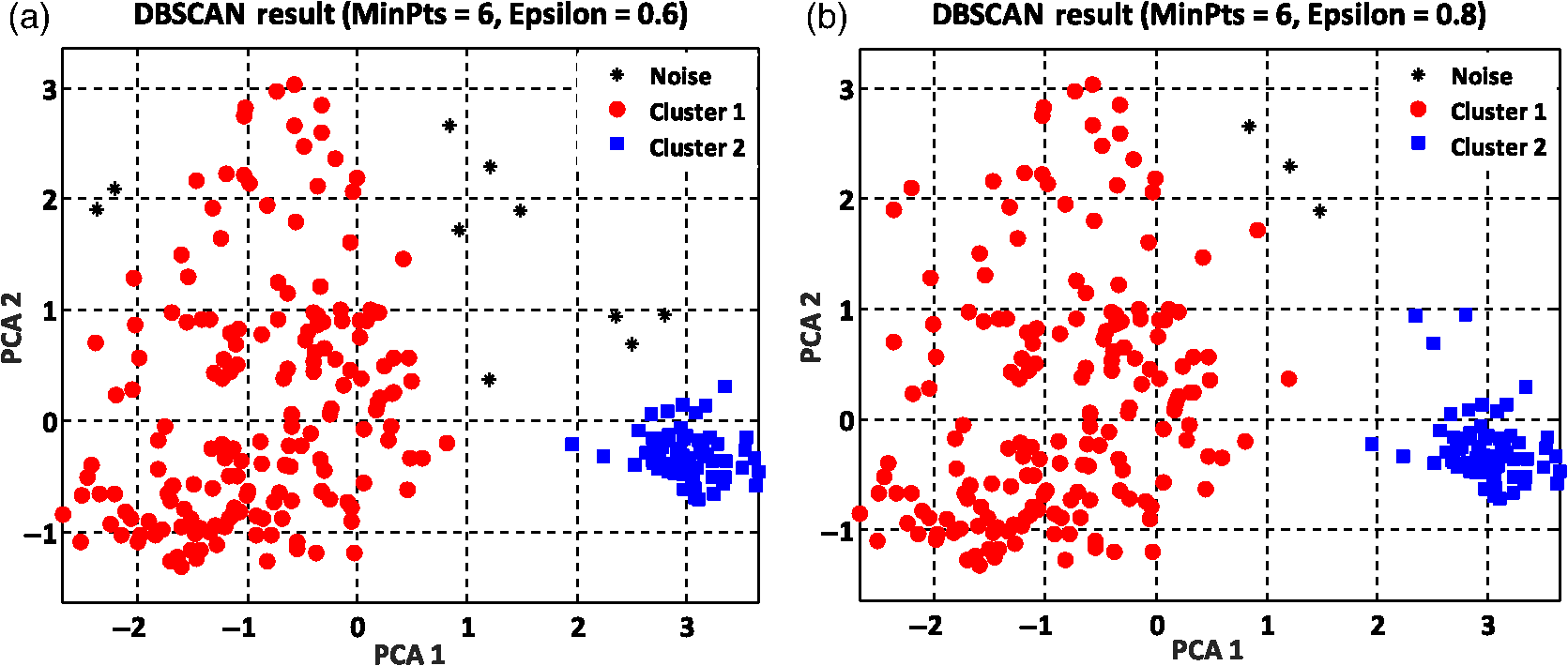
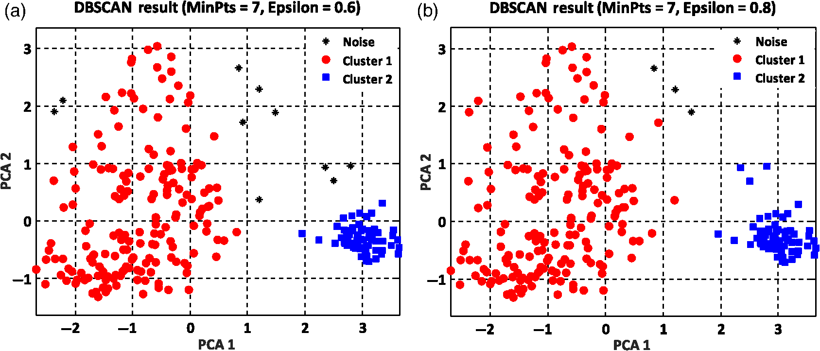
Figure 6 shows the graphical representations of the DBSCAN clustering results for a MinPts value of 4 and epsilon values of 0.6 and 0.8. The DBSCAN clustering performance results for MinPts values of 5, 6, and 7, and epsilon values of 0.6 and 0.8 are also graphically represented in Figs. 7Fig. 8–9, respectively. It is noted that the DBSCAN algorithm that is based on the density of RBC samples in feature space clusters two main RBC types of biconcave and stomatocyte in the same cluster because of their similarities and distinguishes them from the sphero-echinocyte RBC type. In some cases, by changing the epsilon and MinPts value, some of RBCs are considered unknown and marked as noise. It is evident from Fig. 6(b) that we attained a 100% clustering result for the two clusters using a MinPts of 4 and radius of 0.8 and all data points are affected by the radius and MinPts parameters. For the three clusters, according to the density of data points distributed in feature space, the data points of biconcave and sphero-echinocytes are placed in very close proximity to each other. Different radii affect both types and will accordingly be clustered as one cluster. Therefore, we applied the DBSCAN algorithm to cluster RBCs into two clusters.

Fig. 6

Density-based clustering results using MinPts of 4 and epsilon of (a) 0.6 and (b) 0.8.

Fig. 7

Density-based clustering results using MinPts of 5 and epsilon of (a) 0.6 and (b) 0.8.

Fig. 8

Density-based clustering results using MinPts of 6 and epsilon of (a) 0.6 and (b) 0.8.

Fig. 9

Density-based clustering results using MinPts of 7 and epsilon of (a) 0.6 and (b) 0.8.

Different evaluations of the density-based clustering method for different values of epsilon and MinPts, including max iteration, clustering accuracy, and misclassification ratio to cluster all data points in the region of epsilon (radius), as well as number of points far from the other data, which are considered as noise points, are presented in Table 3.

8.2.

k-Medoids Clustering Results

In this experiment, we applied the $k$-medoids clustering method. We plotted the original RBC data distribution using three PCAs to analyze the clustering performance in 3-D-space based on the best 2-D and 3-D features (see Fig. 10).

Fig. 10

Original data distribution in 3-D data space based on the three PCAs using (a) best selected feature set and (b) 2-D features.

We applied $k$-medoids on the 3-D data points based on the three PCAs to cluster RBC data into two and three clusters. For the two clusters, it is observed that the RBC data have been clustered effectively and with high accuracy. As shown in Fig. 11, the $k$-medoids clustering method found the best central data point in which it can perfectly represent all data points in a specific cluster and marked it as medoid point. The data point that has close distance to the medoid point is allocated to that specific cluster. Because of the similarity between the two main types of biconcave and stomatocyte morphologies, their central point, or so-called medoid point, considers them to be one cluster. Figure 11(a) demonstrates that the sphero-echinocyte RBC samples, which are represented as cluster 1, are fully separated from the biconcave and stomatocyte morphologies using the best 2-D- and 3-D-selected features. Figure 11(b) shows a graphical representation of the $k$-medoid clustering method using the 2-D features to cluster RBC samples into two clusters. The clustering accuracy for both the best features and 2-D features is presented in Table 4.

Fig. 11

$k$-medoids clustering results of clustering RBC samples into two clusters using (a) best selected feature set and (b) 2-D features.

Table 4

k-medoids clustering results for two and three clusters on three main types of RBC samples using the best selected features and 2-D features (275 total samples).

Clustering method	Number of clusters	Total misclassified samples	Clustering accuracy rate (%)
$k$-medoids clustering results using 2-D features	2	25	90.9
	3	43	84.3
$k$-medoids clustering results using best selected features	2	4	98.5
	3	14	94.9

Similarly, we also applied the $k$-medoids clustering method to cluster RBC data into three clusters according to the three main RBC types. A graphical representation of the $k$-medoids clustering method on the best features and 2-D features is shown in Fig. 12. The medoid points are circled and indicate the center data point for each cluster (see Fig. 12). The experimental results demonstrate that the three main types of RBC samples can effectively be clustered with a high accuracy using the best features. The clustering accuracy of the $k$-medoids clustering method on 2-D features is presented in Table 4.

Fig. 12

$k$-medoids clustering results and medoid points for clustering RBC samples into three clusters using (a) best selected feature set and (b) 2-D features.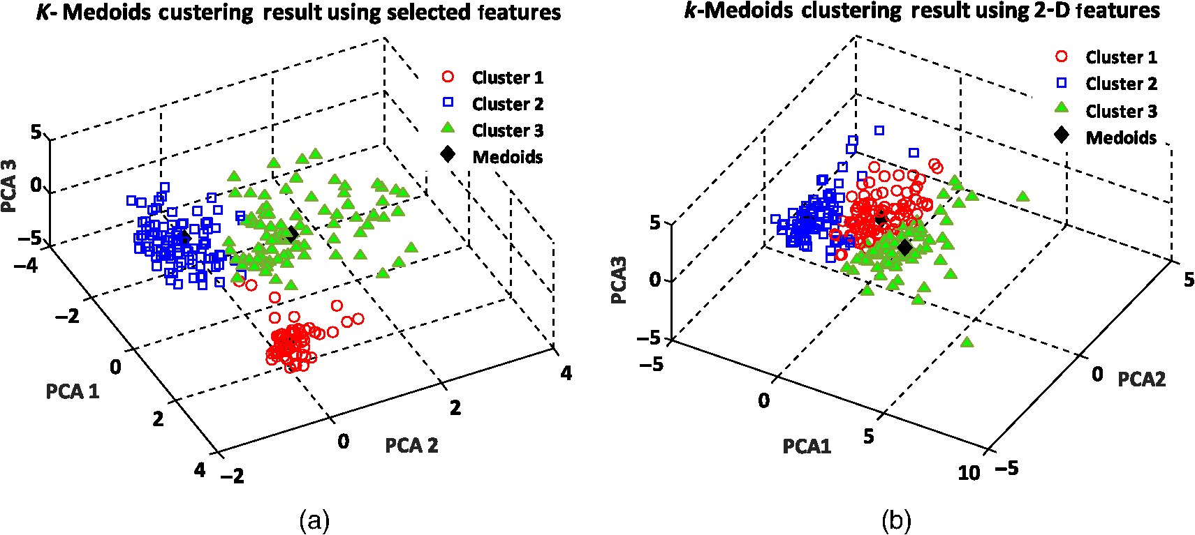

According to Table 4, the clustering accuracy of the best selected features is much higher than using only the 2-D features. This fact proves that 2-D features cannot suitably discriminate between the different RBC types. As shown in Table 4, since two RBC types of biconcave and stomatocyte have some similarities in shape and features, when we increase the number of clusters, some samples are misclassified and cause a decrease in the clustering accuracy for three clusters.

8.3.

k-Means Clustering Results

In the first experiment, the $k$-means clustering method is utilized by defining two numbers of clusters for the RBC data. Figure 13(a) shows the $k$-means clustering results for clustering RBC types using the best features for the two clusters. As we expected, the clustering results demonstrate that $k$-means clusters two RBC types of biconcave and stomatocyte into one cluster because of their similarities and separates them from the sphero-echinocyte RBC type. Figure 13(b) shows a graphical representation of the $k$-means clustering method on 2-D features of the RBC data. The accuracy ratio of both methods is presented in Table 5.

Fig. 13

$k$-means clustering results on RBC samples for two clusters. Different clusters are represented in different colors using (a) best selected feature set and (b) 2-D features.

Table 5

k-means clustering results on three main types of RBC samples for two and three clusters using the best selected features and 2-D features (275 total samples).

Clustering method	Number of clusters	Total misclassified samples	Clustering accuracy rate (%)
$k$-means clustering results using 2-D features	2	37	86.5
	3	52	81.0
$k$-means clustering results using best selected features	2	3	98.9
	3	13	95.2

Similarly, we also apply the $k$-means clustering method to the RBC data to cluster data points into three clusters using the best features and 2-D features. Figure 14 indicates that by using the best-selected features, all RBC types of biconcave, discocyte, and stomatocyte can be clustered to a great extent. The clustering accuracy of the 2-D features is significantly lower than that of the best features (see Table 5).

Fig. 14

$k$-means clustering results on three main RBC samples for three clusters using (a) best selected feature set and (b) 2-D features.

As the $k$-means clustering method uses the mean of all data points in the same cluster as the centroid point, the experimental results indicate that the $k$-means method clusters data with a high accuracy level up to 98% for two clusters and 95% for three clusters using the best features. This fact reveals that 3-D features can significantly influence the mean value of data points in the same cluster.

The results obtained by different clustering methods reveal that clustering techniques can be very efficient and accurate if we can choose a good feature set. Specifically, in RBC clustering, the combination of 2-D and 3-D features can significantly increase the accuracy of the clustering results.

9.

Internal Evaluation of Clustering Techniques

In another experiment with internal evaluation of the clustering technique, $k$-means (almost similar results are obtained for the other clustering techniques) is performed by measuring the SI. SI varies between $-1$ and $+1$, and high SI indicates that the input sample is well-matched to its own cluster and poorly matched to neighboring clusters. If most points have a high silhouette value, the plot shows an assessment of how close each sample in one cluster is to samples in the neighboring clusters and using this way, we can measure parameters, such as number of clusters visually.

Silhouette coefficients near $+1$ mean that the samples are well distinguished from neighboring clusters. Samples that are very close to the neighboring clusters will get zero value, and negative values indicate samples are clustered to the wrong cluster. According to Figs. 15(a) and 15(b), we can see that most of the silhouette values are close to $+1$. There are a few values below zero that are not well matched to the corresponding cluster.

Fig. 15

SI for (a) two clusters and (b) three clusters.

10.

Conclusions

The quality and functionality of RBCs play major roles in the human health system. Storing blood for long periods can damage the functionality and quality of RBCs. In this study, we applied several unsupervised clustering methods, including DBSCAN clustering, $k$-medoids, and $k$-means clustering, for clustering three RBC types of biconcave, stomatocyte, and sphero-echinocyte into two and three clusters. The RBC samples that were visualized by the DHM technique were extracted from the blood sample. DHM provides QPIs of the 3-D profile of RBCs with nanometer accuracy. More than 14 2-D and 3-D features were extracted from every RBC sample. We selected a combinational set of 2-D and 3-D features that can suitably discriminate between the three regular RBC types. The combinational features include the ACT, PSA, sphericity coefficient, perimeter, and MCV. The clustering power of the combinational set of 2-D and 3-D features was compared against a set of six 2-D features, and the clustering results were evaluated for every clustering method. The experimental results and performance of clustering methods indicate that the combinational feature set can yield better RBC clustering. In addition, using the combinational features, we were able to cluster biconcave, stomatocyte, and sphero-echinocyte morphologies to a great extent, which are paramount for RBC abnormality analyses and shape-related diseases.