Refractive-index-mismatch induced aberrations in single-photon and two-photon microscopy and the use of aberration correction

Martin J. Booth; Tony Wilson

doi:10.1117/1.1382808

1 July 2001 Refractive-index-mismatch induced aberrations in single-photon and two-photon microscopy and the use of aberration correction

Martin J. Booth, Tony Wilson

Author Affiliations +

Journal of Biomedical Optics, Vol. 6, Issue 3, (July 2001). https://doi.org/10.1117/1.1382808

1. Introduction

Scanning single-photon (1−p) and two-photon (2−p) excitation fluorescence microscopes are becoming ubiquitous tools in the biological sciences.¹ ² ³ Many microscopes can be configured to operate in both 1−p and 2−p fluorescence excitation modes. In 1−p excitation fluorescence microscopy, a fluorophore is excited by a single photon of a particular wavelength, typically from a laser source. The fluorophore then returns to the ground state emitting a photon at a slightly longer fluorescence wavelength, which is separated from the excitation light by a suitable filter and then may be detected by a photodetector. The 2−p excitation process, however, relies on the simultaneous absorption of two, longer wavelength photons, whereafter a fluorescence photon is emitted. The excitation wavelength is typically twice that used in the 1−p case. In 1−p microscopy, the use of a confocal pinhole in the detection path allows axial sectioning and, therefore, three dimensional imaging.⁴ ⁵ In 2−p microscopy, the quadratic dependence of the fluorescence intensity on the illumination intensity means that the fluorescence emission is always confined to the region of the focus—the system possesses an inherent optical sectioning property. A confocal pinhole may however be used, increasing resolution at the expense of signal level.⁶ Benefits of 2−p microscopy in comparison to 1−p microscopy include the use of red or infrared lasers to excite ultraviolet dyes, confinement of photobleaching to the focal region, and the reduced effects of scattering. However, compared with that of 1−p excitation, the fluorescence yield of many fluorescent dyes under 2−p excitation is low.⁷

Theoretical comparisons of resolution between 1−p and 2−p methods have shown that, for a given fluorescent dye and in the absence of aberrations, the resolution of 1−p confocal and 2−p confocal are roughly equivalent, whereas the resolution of 2−p conventional is worse by a factor of approximately 2.⁶ Previous experimental investigations have looked into the effects of refractive index mismatch on the imaging properties of 1−p and 2−p microscopes and shown a decrease in resolution and signal strength as the focusing depth increases.⁸ ⁹ ¹⁰

In this paper, we expand on previous analyses by comparing directly the imaging capabilities, via signal level, lateral, and axial resolution, of 1−p and 2−p microscopes under the effects of spherical aberration induced by a refractive index mismatched interface. We work from the assumption that the fluorescent dye will be the same in both the 1−p and 2−p case, so that the emission wavelength will be the same in both cases. We also investigate the benefits of applying aberration correction which could be performed, for example, in an adaptive microscope.¹¹ Finally, we derive a geometrical optics approximation which describes the axial resolution as a function linear in the focusing depth.

2. The Aberration Function

The pupil function P describes the complex field distribution in the pupil of an objective lens. It is defined in terms of the normalized radial coordinate ρ such that the pupil has a radius of 1. The pupil function is a useful way of describing any aberrations introduced into the system. In an unaberrated system, P=1. We consider the situation when the objective lens is used to focus through an interface between media with different refractive indices. This is described schematically in Figure 1. The distance d is the nominal focusing depth, i.e., the depth of the focus in a matched medium. Gibson and Lanni¹² investigated focusing through such an interface and expressed the phase aberration as a function in the pupil plane. We have shown previously¹³ that their expressions can be simplified so that when focusing a nominal depth d into a medium of refractive index n₂ from a medium of refractive index n₁, the phase aberration is given by

Eq. (1)

Ψ (ρ, d) = d \frac{2 π}{λ} n_{1} sin α_{1} [\sqrt{{csc}^{2} α_{2} - ρ^{2}} - \sqrt{{csc}^{2} α_{1} - ρ^{2}}],

where α₁ is the semiaperture angle of the objective lens and α₂ is found using Snell’s law: n₁ sin α₁ =n₂ sin α₂. The corresponding pupil function is therefore given by

Eq. (2)

P (ρ, d) = exp [j Ψ (ρ, d)] .

To¨ro¨k et al.;¹⁴ showed that the aberration function can be expanded as an infinite but rapidly converging series of zero order (radially symmetric) Zernike polynomials. The Zernike polynomials are an orthogonal set of polynomials defined over the unit circle which, in general, consist of a radial polynomial multiplied by an azimuthal term. We refer to the polynomials as Z_n,m(⋅) where n and m are the radial and azimuthal orders, respectively. The aberration function can be expanded in terms of the Zernike polynomials for which m=0, that is

Eq. (3)

Ψ (ρ, d) = d \frac{2 π}{λ} n_{1} sin α_{1} [\sum_{\begin{matrix} n = 0 \\ n even \end{matrix}}^{\infty} A_{n, 0} Z_{n, 0} (ρ)],

where the Zernike polynomials are defined as

Eq. (4)

Z_{n, 0} (ρ) = \sqrt{n + 1} \sum_{s = 0}^{n / 2} \frac{{(- 1)}^{s} (n - s)!}{s! {(n / 2 - s)!}^{2}} ρ^{n - 2 s} for n even .

The condition in the summation of Eq. (3) that n is even is a consequence of the fact that Z_n,0 is undefined for n odd. The coefficients A_n,0 are functions of the angles α₁ and α₂ and are given by¹³

Eq. (5)

A_{n, 0} = B_{n} (α_{1}) - B_{n} (α_{2}),

where

Eq. (6)

B_{n} (γ) = [1 - (\frac{n - 1}{n + 3}) {tan}^{4} (\frac{γ}{2})] \frac{{tan}^{n - 1} (\frac{γ}{2})}{2 (n - 1) \sqrt{n + 1}} .

The functional forms of Z_n,0(ρ) are shown in Table 1 together with the aberration which they describe. Mathematically, the role of aberration correction is to modify the phase in the pupil plane by subtracting specific amounts of aberration so that the phase becomes closer to the ideal P(ρ,d)=1, unaberrated case. We will assume that it is possible to totally remove any chosen Zernike mode or modes from the aberration function so that the pupil plane phase is described by the “corrected” phase function Ψ^′(ρ,d):

Figure 1

The focusing geometry showing the refraction of rays at the interface between two media of different refractive index.

Table 1

Radially symmetric Zernike polynomials for n=0, 2, 4, 6 & 8.
n	Z_n ⁰(ρ)	Description
0	1	Piston
2	√3(2ρ²−1)	Defocus
4	$\sqrt{5} (6 ρ^{4} - 6 ρ^{2} + 1)$	1st order spherical aberration
6	$\sqrt{7} (20 ρ^{6} - 30 ρ^{4} + 12 ρ^{2} - 1)$	2nd order spherical aberration
8	$\sqrt{9} (70 ρ^{8} - 140 ρ^{6} + 90 ρ^{4} - 20 ρ^{2} + 1)$	3rd order spherical aberration

Eq. (7)

Ψ^{'} (ρ, d) = Ψ (ρ, d) - d \frac{2 π}{λ} n_{1} sin α_{1} [\sum_{\begin{array}{l} n = 0 \\ n e v e n \end{array}}^{2 N + 2} A_{n, 0} Z_{n, 0} (ρ)] .

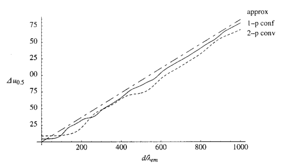
The constant N describes the degree of correction. The corresponding pupil function is given by

Eq. (8)

P (ρ, d) = exp [j Ψ^{'} (ρ, d)] .

Equation (7) is formulated so that when N=0 both Z_0,0 and Z_2,0 are corrected. The mode Z_0,0 describes piston, a constant phase shift across the wave front, which has no effect on the aberrated point spread function. The next mode Z_2,0 represents defocus, which simply creates an axial shift in the intensity distribution of the focus. In a microscope, this corresponds to a movement of the specimen relative to the objective and so is unimportant in our analysis. The removal of these two modes from the aberration function does, however, have considerable beneficial effect on the accuracy of later calculations.

3. The Point Spread Function

When the pupil function is rotationally invariant, the intensity in the region of the focus of an objective lens can be described by the equation⁴

Eq. (9)

I (ν, u, d) = {| \int_{0}^{1} P (ρ, d) exp (j \frac{u}{2} ρ^{2}) J_{0} (ρ ν) ρ d ρ |}^{2},

where J₀(⋅) is the zeroth order Bessel function of the first kind, P(⋅) is the pupil function of the lens, and ρ is the radial coordinate in the pupil plane, normalized such that the pupil has unity radius. The normalized lateral and axial coordinates ν and u are given by

Eq. (10)

ν = \frac{2 πnr}{λ} sin α,

Eq. (11)

u = \frac{8 πnz}{λ} {sin}^{2} (\frac{α}{2}),

where r and z are the radial and axial displacements from the nominal focus, λ is the free space wavelength of the illumination light, and n is the refractive index of the immersion medium. α is the semiaperture angle of the objective lens and is related to the numerical aperture (NA) by NA=n sin α.

In a fluorescence microscope, one normally chooses a particular fluorophore for a given application and the emission wavelength is dictated by this choice. When comparing the performance of 1−p and 2−p microscopes it is therefore logical to assume that the emission wavelength is the same in both cases. The reader should be wary that some authors use the same excitation wavelength which can give misleading results when comparing achievable resolution. We assume that the fluorescence emission will be at a single wavelength, given by λ_em, irrespective of the mode of excitation. The wavelength required for 1−p excitation is generally shorter than the emission wavelength so it can be written as βλ_em, where β<1. 2−p excitation requires the simultaneous absorption of two photons of half the energy, so we take the excitation wavelength in this case to be 2βλ_em. Measurements by Xu et al.;¹⁵ show that this is a reasonable approximation for many fluorescent dyes. We now define the normalized coordinated in terms of λ_em by making the substitution λ=λ_em in Eqs. (10) and (11) so that

Eq. (12)

ν = \frac{2 πnr}{λ_{em}} sin α,

Eq. (13)

u = \frac{8 πnz}{λ_{em}} {sin}^{2} (\frac{α}{2}) .

Using Eqs. (9), (12), and (13) we can write expressions for the effective point spread functions (PSFs) of the different imaging modes taking into account the differences in wavelength between the excitation and fluorescence in each case. This involves scaling the lateral and axial coordinates as well as the size of the aberration. We use the subscripts 1p and 2p to refer to single and two photon excitation. The subscripts conv and conf refer to conventional and confocal imaging, respectively

Eq. (14)

I_{1 p - conv} (ν, u, d) = I (\frac{ν}{β}, \frac{u}{β}, \frac{d}{β}),

Eq. (15)

I_{1 p - conf} (ν, u, d) = I (\frac{ν}{β}, \frac{u}{β}, \frac{d}{β}) I (ν, u, d),

Eq. (16)

I_{2 p - conv} (ν, u, d) = I^{2} (\frac{ν}{2 β}, \frac{u}{2 β}, \frac{d}{2 β}),

Eq. (17)

I_{2 p - conf} (ν, u, d) = I^{2} (\frac{ν}{2 β}, \frac{u}{2 β}, \frac{d}{2 β}) I (ν, u, d) .

Equations (14 15 16 17) are similar to those derived by Gu and Sheppard.⁶ We now look at Eqs. (15) and (16) when β=1:

Eq. (18)

I_{1 p - conf} (ν, u, d) = I^{2} (ν, u, d),

Eq. (19)

I_{2 p - conv} (ν, u, d) = I^{2} (\frac{ν}{2}, \frac{u}{2}, \frac{d}{2}) .

At zero focusing depth (d=0), the longer excitation wavelength in 2−p conventional microscopy results in a PSF which is twice as large as the 1−p confocal PSF in both the lateral and axial dimensions. This wavelength difference also means that the aberration suffered by 2−p conventional is only half that suffered by 1−p confocal at a given focusing depth. As we show later in this paper, these two effects balance out so that under large aberrations the PSFs in the two imaging modes are approximately the same size.

4. Resolution Measurements

It is always desirable to find a simple way of describing the imaging properties of a microscope, for example, via the concept of resolution. Numerous criteria have been suggested for calculating the resolution of scanning microscopes, for example, the full-width half-maximum (FWHM) of the effective PSF or the gradient of the axial response to a semi-infinite fluorescent sea (see, e.g., Refs. 16 and 5). Most of these have been formulated for describing imaging capabilities with unaberrated PSFs in mind. For this reason, they are not always useful when describing heavily aberrated PSFs. The FWHM measurement, for example, only has useful meaning when the PSF consists of a single, reasonably symmetric main peak with negligible sidelobes. It gives misleading results when the aberrations are large. Since aberrated PSFs are often highly asymmetric, we require a measurement which provides some indication of the spatial spread of the PSF. For axial resolution, we do this by finding the distance between the two lateral planes, between which a chosen proportion ɛ of the total integrated fluorescence W(d) in the PSF is enclosed. In other words, we define axial resolution as

Eq. (20)

Δ u_{ɛ} = u_{2} - u_{1},

where u₁ and u₂ are defined by

Eq. (21)

\int_{- \infty}^{u 1} \int_{0}^{\infty} I_{mode} (ν, u, d) ν d ν du = \frac{(1 - ɛ)}{2} W (d),

Eq. (22)

\int_{- \infty}^{u 2} \int_{0}^{\infty} I_{mode} (ν, u, d) ν d ν du = \frac{(1 + ɛ)}{2} W (d) .

I_mode represents any of the PSFs described in Eq. (14 15 16 17) and W(d) is the total integrated fluorescence in the PSF:

Eq. (23)

W (d) = \int_{- \infty}^{\infty} \int_{0}^{\infty} I_{mode} (ν, u, d) ν d ν du .

As an example, for ɛ=0.5, Δu_ɛ is the width of the middle 50 of the axial scan of a fluorescent plane through the PSF. Alternatively, it is the distance between the 25 and 75 points on the axial response curve to a semi-infinite fluorescent sea.¹⁷ See Figure 2 for illustration. As is well known, the 1−p conventional axial response to a fluorescent plane is constant for all u and, therefore, Δu_ɛ is undefined.

Figure 2

The axial response of a confocal microscope to: (a) a defocused fluorescent plane and (b) a semi-infinite fluorescent sea. The response curve of (b) is simply the integral of that in (a). The central 50 of the area under the former curve therefore corresponds to the region between the 25 and 75 points of the latter curve.

As a measurement of lateral resolution, we define v_ɛ by

Eq. (24)

\int_{0}^{v_{e}} \int_{- \infty}^{\infty} I_{mode} (ν, u, d) du ν d ν = ɛ W (d) .

Therefore, for ɛ=0.5, v_ɛ represents the radius of the infinite cylinder centered on the optical axis which contains half of the total integrated fluorescence.

5. Results and Discussion

In this section, we compare the properties of 1−p confocal, 2−p conventional, and 2−p confocal scanning microscopes. We do not consider 1−p conventional since its lack of axial sectioning is well known. For these calculations, we consider an oil immersion objective of NA=0.9 focusing into a medium of refractive index n₂=1.33. The oil is taken to have a refractive index n₁=1.5. Initially we do not perform any aberration correction, i.e., N=0 in Eq. (7). The wavelength ratio β is taken to be unity and we express the focusing depth d in terms of λ_em.

Figure 3 shows W(d), the integrated fluorescence from the aberrated PSFs for each imaging mode when focusing a depth d into the second medium. Each curve is normalized to its value at d=0. For the purpose of the calculations, it was assumed that the whole PSF lies within fluorescent material. This assumption is inaccurate in the region of d=0, although the effects on this scale are not noticeable. All three modes suffer decreased intensity when focusing deep into the second medium. 2−p conventional is least affected, although 2−p confocal suffers most, dropping to around 10 at d=200λ_em. The reader must be wary of the normalization used here. Many other factors not considered here contribute to the overall signal level in a real microscope and absolute comparison between imaging modes should not be inferred from these results. For a given aberration, the signal level for 2−p confocal, for example, would always be considerably lower than 2−p conventional in any system.

Figure 3

The integrated fluorescence as a function of focusing depth for each of the three imaging modes 1−p confocal (solid line), 2−p conventional (short dashed line), and 2−p confocal (long dashed line).

Figure 4 shows the axial resolution, Δu_0.5, as a function of d. It is clear that for 2−p confocal the resolution is superior (albeit at the expense of vastly reduced signal). What is more interesting are the results for 1−p confocal and 2−p conventional. It is well known that the longer excitation wavelength required for 2−p microscopy results in a larger PSF when no aberration is present (see e.g., Ref. 6). This can be seen for low values of d. However, Eq. (1) shows that the magnitude of the induced aberration varies inversely with wavelength. The aberration is therefore smaller at the longer 2−p excitation wavelength. The combination of these effects results in the behavior seen for d>100λ_em, where Δu_0.5 is almost the same for both 1−p confocal and 2−p conventional. In fact, when β=1, the two curves are identical except for scaling of the axes.

Figure 4

The axial resolution Δu_0.5 as a function of focusing depth.

Figure 5 shows the lateral resolution v_0.5. At small focusing depths, 1−p confocal and 2−p confocal have similar lateral resolution, whereas for 2−p conventional it is approximately twice the size. At higher values of d, the best lateral resolution is seen for 2−p confocal, where it only increases marginally over the range of depths shown. For 1−p confocal and 2−p conventional, the values of v_0.5 increase at a similar rate meaning that 1−p confocal always demonstrates better lateral resolution.

Figure 5

The lateral resolution v_0.5 as a function of focusing depth.

We now perform aberration correction and remove one order of spherical aberration (N=1). The corresponding plots of W(d) are shown in Figure 6. With this correction, the intensity is partially restored. Again, 2−p conventional shows the least decrease in intensity; 2−p confocal is still affected the most although it only decreases to around 70 at d=500λ_em.

Figure 6

The integrated fluorescence as a function of focusing depth with correction for one Zernike mode (N=1).

The variation in Δu_0.5 is shown in Figure 7 for the corrected PSFs. There is very little increase in Δu_0.5 for either 2−p mode in this range. For 1−p confocal, there is a slight increase owing to the larger phase aberration suffered by the shorter wavelength.

Figure 7

The axial resolution Δu_0.5 as a function of focusing depth with correction for one Zernike mode (N=1).

Figure 8 shows the lateral resolution v_0.5. With the correction, there is very little change in v_0.5 for any of the modes within this range. We see that 1−p confocal and 2−p confocal have almost the same resolution, which is around half the resolution for 2−p conventional.

Figure 8

The axial resolution v_0.5 as a function of focusing depth with correction for one Zernike mode (N=1).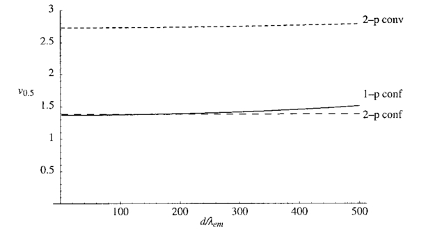

These resolution results are calculated for an NA of 0.9, around the limit of accuracy for the Fourier based theory of focusing. We can expect, however, that the general trends observed will be seen for higher NAs and different values of refractive index. Figure 9 shows a logarithmic plot of the Zernike mode coefficients of Eq. (5) as a function of NA, for n=4, 6, and 8. This shows that the aberration function of Eq. (1) is dominated by first order spherical aberration for lower NAs, where correction of one mode is sufficient. At higher NAs, it would be necessary to correct for more Zernike terms to obtain an equivalent level of correction at the same focusing depth.

Figure 9

Zernike mode coefficients as a function of NA:n=4 (solid line), n=6 (short dashed line), and n=8 (long dashed line).

6. Estimation of the Axial Resolution

When the aberrations are large, the Fourier integrals of Eqs. (14 15 16 17) require a large number of integration points and therefore a long calculation time. It is, however, possible to approximate the behavior of the effective PSF by geometrical optics. Geometrical optics is equivalent to wave optics in the limit that λ→0 so that diffraction and interference effects are negligible. The behavior of light can be described by rays that travel in a direction normal to the wavefronts we have considered so far in this analysis. In a focusing system free from aberrations, the rays pass through the pupil parallel to the optic axis and are focused by the objective lens so that all rays pass through the focal point on the axis. In an aberrated system, the rays are, in general, nonparallel when passing through the pupil and no longer pass through the focal point but are spread out, intersecting the optic axis at different axial distances. By ascertaining the directions of the rays, we can easily calculate the on-axis intensity distribution of the focus. We consider a simpler definition of axial resolution based upon the on-axis intensity only. Equations (20 21 22 23) are recast so that

Eq. (25)

Δ u_{ɛ} = u_{2} - u_{1},

where u₁ and u₂ are defined by

Eq. (26)

\int_{- \infty}^{u_{1}} I_{mode} (0, u, d) du = \frac{(1 - ɛ)}{2} \int_{- \infty}^{\infty} I_{mode} (0, u, d) du,

Eq. (27)

\int_{- \infty}^{u_{2}} I_{mode} (0, u, d) du = \frac{(1 + ɛ)}{2} \int_{- \infty}^{\infty} I_{mode} (0, u, d) du .

We now show that the integrals in Eqs. (26) and (27) can be transformed into integrals in the pupil plane and then that Δu_ɛ∝d.

We rewrite the integral of Eq. (9), which describes the focal intensity, as

Eq. (28)

I (ν, u, d) = | \int_{0}^{1} exp{j Φ(ρ, u, d)} J_{0} (ρ ν) ρ d ρ |^{2},

where the phase function Ф combines the previous aberration function Ψ and the quadratic defocus term

Eq. (29)

Φ (ρ, u, d) = Ψ (ρ, d) + \frac{u}{2} ρ^{2} .

A ray passing through the pupil at a given radius ρ will only pass through the focal point if it is parallel to the optic axis at the pupil; in other words, when the wave front gradient is zero:

Eq. (30)

\nabla Φ (ρ, u, d) = \frac{\partial}{\partial ρ} Φ (ρ, u, d) = 0 .

Substituting Eq. (29) into Eq. (30) and using Eq. (1), we find that

Eq. (31)

u (ρ) = \frac{2 π NA d}{λ} (\frac{1}{\sqrt{{csc}^{2} α_{2} - ρ^{2}}} - \frac{1}{\sqrt{{csc}^{2} α_{1} - ρ^{2}}}) .

This equation relates the radius ρ at which the ray passes through the pupil to the axial coordinate u at which it crosses the optic axis in the region of the focus. Inspection of this equation shows that there is a one to one relationship between u and ρ in the range 0⩽ρ⩽1. We can therefore relate the on-axis intensity near the focus to the intensity in the pupil. It will be useful later if we define a new function u^′(ρ), which is independent of d, so that we can write Eq. (31) as

Eq. (32)

u (ρ) = d u^{'} (ρ) .

An annular element of the pupil of width dρ will illuminate an element of the optic axis du with intensity 2πρU(ρ)dρ, where U(ρ) is the intensity distribution in the pupil. As in the rest of the paper, we take U(ρ)=1. The element of on-axis intensity U(u)du can be written

Eq. (33)

U (u) d u = 2 π ρ d ρ,

which allows us to transform the integrals in Eqs. (26) and (27). For both 1−p confocal and 2−p conventional, the detected fluorescence is proportional to the square of the illumination intensity, so the integral on the left hand side of Eq. (26) becomes

Eq. (34)

\begin{matrix} \int_{- \infty}^{u_{1}} U^{2} (u) d u & = & \int_{0}^{u_{1}} {(2 π ρ \frac{d ρ}{d u})}^{2} d u \\ = & 4 π^{2} \int_{0}^{ρ_{1}} ρ^{2} {(\frac{d u}{d ρ})}^{- 1} d ρ, \end{matrix}

where ρ₁ and u₁ are related via Eq. (31). The other integrals can be transformed in a similar manner. Substituting for u^′(ρ) using Eq. (32), Eq. (26) then becomes

Eq. (35)

\frac{4 π^{2}}{d} \int_{0}^{ρ_{1}} ρ^{2} {(\frac{d u^{'}}{d ρ})}^{- 1} d ρ = \frac{2 π^{2} (1 - ɛ)}{d} \int_{0}^{1} ρ^{2} {(\frac{d u^{'}}{d ρ})}^{- 1} d ρ .

Similarly, Eq. (27) becomes

Eq. (36)

\frac{4 π^{2}}{d} \int_{0}^{ρ_{2}} ρ^{2} {(\frac{d u^{'}}{d ρ})}^{- 1} d ρ = \frac{2 π^{2} (1 + ɛ)}{d} \int_{0}^{1} ρ^{2} {(\frac{d u^{'}}{d ρ})}^{- 1} d ρ .

It can be seen that neither ρ₁ nor ρ₂ depends on d. From Eqs. (32) and (25) it is easily shown that

Eq. (37)

Δ u_{ɛ} = d {u^{'} (ρ_{2}) - u^{'} (ρ_{1})} .

This is plotted in Figure 10 alongside the full, Fourier calculations of Δu_0.5 for 1−p confocal and 2−p conventional. This geometrical optics approximation is inaccurate for low values of d since it neglects diffraction effects. However, when the aberrations are larger, we see that it provides a good estimate of the axial extent of the PSF.

Figure 10

Axial resolution Δu_0.5 as a function of focusing depth: 1−p confocal (solid line), 2−p conventional (short dashed line), and geometrical optics approximation (dot dash line).

6. Conclusion

We have investigated the effects of refractive index mismatch induced spherical aberration on the signal strength and resolution in 1−p confocal, 2−p conventional, and 2−p confocal scanning microscope configurations. We have also shown the benefits obtained by removing Zernike spherical aberration, something which may be implemented in an adaptive microscope. Without correction, 2−p confocal demonstrates superior axial and lateral resolution although it must be remembered that the overall signal level will always be vastly lower than in the other imaging modes. More importantly, we have shown that, except for at shallow focusing depths, the axial resolution of 1−p confocal and 2−p conventional microscopes are very similar and the resolution scales linearly with depth. With aberration correction, the signal strength can be restored and the best axial and lateral resolution is achieved with 1−p confocal or 2−p confocal microscopes.

Acknowledgment

This work is supported by the Biotechnology and Biological Sciences Research Council, UK.

REFERENCES

1.

W. Denk , J. H. Strickler , and W. W. Webb , “Two-photon laser scanning confocal microscopy,” Science , 248 73 –76 (1990). Google Scholar

2.

Handbook of Biological Confocal Microscopy, J. B. Pawley, Ed. Plenum, New York (1995).

3.

K. Ko¨nig , “Multiphoton microscopy in life sciences,” J. Microsc. , 200 (2), 83 –104 (2000). Google Scholar

4.

T. Wilson and C. J. R. Sheppard, Theory and Practice of Scanning Optical Microscopy, Academic, London (1984).

5.

Confocal Microscopy, T. Wilson, Ed. Academic, London (1990).

6.

M. Gu and C. J. R. Sheppard , “Comparison of three-dimensional imaging properties between two-photon and single-photon fluorescence microscopy,” J. Microsc. , 177 (2), 128 –137 (1995). Google Scholar

7.

C. Xu and W. W. Webb , “Measurement of two-photon excitation cross sections of molecular fluorophores with data from 690 to 1050 nm,” J. Opt. Soc. Am. B , 13 (3), 481 –491 (1996). Google Scholar

8.

S. W. Hell , G. Reiner , C. Cremer , and E. H. K. Stelzer , “Aberrations in confocal fluorescence microscopy induced by mismatches in refractive index,” J. Microsc. , 169 (3), 391 –405 (1993). Google Scholar

9.

H. Jacobsen , P. Ha¨nninen , E. Soini , and S. W. Hell , “Refractive-index-induced aberrations in two-photon confocal fluorescence microscopy,” J. Microsc. , 176 (3), 226 –230 (1994). Google Scholar

10.

C. J. de Grauw , J. M. Vroom , H. T. M. van der Voort , and H. C. Gerritsen , “Imaging properties in two-photon excitation microscopy and effects of refractive-index mismatch in thick specimens,” Appl. Opt. , 38 (28), 5995 –6003 (1999). Google Scholar

11.

M. A. A. Neil , R. Juskaitis , M. J. Booth , T. Wilson , T. Tanaka , and S. Kawata , “Adaptive aberration correction in a two-photon microscope,” J. Microsc. , 200 (2), 105 –108 (2000). Google Scholar

12.

S. F. Gibson and F. Lanni , “Experimental test of an analytical model of aberration in an oil-immersion objective lens used in three-dimensional microscopy,” J. Opt. Soc. Am. A , 8 (10), 1601 –1613 (1991). Google Scholar

13.

M. J. Booth , M. A. A. Neil , and T. Wilson , “Aberration correction for confocal imaging in refractive index mismatched media,” J. Microsc. , 192 (2), 90 –98 (1998). Google Scholar

14.

P. To¨ro¨k , P. Varga , and G. Ne´meth , “Analytic solution of the diffraction integrals and interpretation of wave-front distortion when light is focussed through a planar ianterface between materials of mismatched refractive indices,” J. Opt. Soc. Am. , 12 2660 –2671 (1995). Google Scholar

15.

C. Xu , R. M. Williams , W. Zipfel , and W. W. Webb , “Multiphoton excitation cross-sections of molecular fluorophores,” Bioimaging , 4 (3), 198 –207 (1996). Google Scholar

16.

M. Gu, Principles of Three-Dimensional Imaging in Confocal Microscopes, World Scientific, Singapore (1996).

17.

R. W. Wijnaendts-van-Resandt , H. J. B. Marsman , R. Kaplan , J. Davoust , E. H. K. Stelzer , and R. Stricker , “Optical fluorescence microscopy in three dimensions: microtomoscopy,” J. Microsc. , 138 29 –34 (1985). Google Scholar

Notes

Address all correspondence to M. J. Booth. E-mail: martin.booth@eng.ox.ac.uk

Citation Download Citation

Martin J. Booth and Tony Wilson "Refractive-index-mismatch induced aberrations in single-photon and two-photon microscopy and the use of aberration correction," Journal of Biomedical Optics 6(3), (1 July 2001). https://doi.org/10.1117/1.1382808

Published: 1 July 2001

Access the abstract

JOURNAL ARTICLE
7 PAGES

DOWNLOAD PAPER SAVE TO MY LIBRARY

GET CITATION

CITATIONS

Cited by 85 scholarly publications.

Explore citations on Lens.org

RIGHTS & PERMISSIONS

Get copyright permission Get copyright permission on Copyright Marketplace

KEYWORDS

Confocal microscopy

Point spread functions

Luminescence

Microscopes

Aberration correction

Refractive index

Geometrical optics

1.

Introduction

2.

The Aberration Function